Configuring Your Simulation

This example demonstrates how to customize simulation parameters using keyword arguments. You can override any default parameter to explore different economic scenarios.

BAM Engine uses a three-tier configuration system: 1. Package defaults 2. User config file (YAML) 3. Keyword arguments (highest priority, shown here)

Basic Configuration

The simplest way to configure a simulation is to pass parameters as keyword arguments to Simulation.init().

import bamengine as bam

# Create simulation with custom agent counts
sim = bam.Simulation.init(
    n_firms=200,  # Double the default
    n_households=1000,  # More households
    n_banks=20,  # More banks
    seed=42,
)

print("Custom configuration:")
print(f"  Firms: {sim.n_firms}")
print(f"  Households: {sim.n_households}")
print(f"  Banks: {sim.n_banks}")

Custom configuration:
  Firms: 200
  Households: 1000
  Banks: 20

Economic Parameters

Customize economic parameters to explore different scenarios. Here we create a low-friction economy with different shock widths.

sim_low_friction = bam.Simulation.init(
    n_firms=100,
    n_households=500,
    # Shock width parameters
    h_rho=0.05,  # Lower production shock (default: 0.10)
    h_xi=0.02,  # Lower wage shock (default: 0.05)
    # Labor market parameters
    theta=4,  # Shorter base contract duration (default: 8)
    # Search friction parameters
    max_M=6,  # More job applications per worker (default: 4)
    max_H=4,  # More loan applications per firm (default: 2)
    seed=42,
)

print("\nLow-friction economy parameters:")
print(f"  Production shock (h_rho): {sim_low_friction.config.h_rho}")
print(f"  Wage shock (h_xi): {sim_low_friction.config.h_xi}")
print(f"  Contract duration (theta): {sim_low_friction.config.theta}")

Low-friction economy parameters:
  Production shock (h_rho): 0.05
  Wage shock (h_xi): 0.02
  Contract duration (theta): 4

Initial Conditions

You can also customize initial conditions for agents. Parameters can be either scalars (applied to all agents) or arrays (agent-specific values).

# Custom initial conditions with higher firm net worth
sim_wealthy_firms = bam.Simulation.init(
    n_firms=100,
    n_households=500,
    net_worth_init=200.0,  # All firms start with 200 (default: 1.0)
    price_init=2.0,  # Higher initial prices (default: 1.5)
    savings_init=5.0,  # Households start with more savings (default: 3.0)
    seed=42,
)

# Access roles via get_role() for cleaner API
bor = sim_wealthy_firms.get_role("Borrower")
prod = sim_wealthy_firms.get_role("Producer")
con = sim_wealthy_firms.get_role("Consumer")

print("\nCustom initial conditions:")
print(f"  Initial firm net worth: {bam.ops.mean(bor.net_worth):.1f}")
print(f"  Initial prices: {bam.ops.mean(prod.price):.1f}")
print(f"  Initial household savings: {bam.ops.mean(con.savings):.1f}")

Custom initial conditions:
  Initial firm net worth: 200.0
  Initial prices: 2.0
  Initial household savings: 5.0

Compare Scenarios

Run two simulations with different parameters and compare outcomes. We use sim.run() with collection to properly track unemployment.

import numpy as np

# Baseline scenario
sim_baseline = bam.Simulation.init(n_firms=100, n_households=500, seed=42)
baseline_results = sim_baseline.run(
    n_periods=100,
    collect={
        "Worker": ["employed"],
        # Capture employment after production (steady-state, before bankruptcy resets)
        "capture_timing": {"Worker.employed": "firms_run_production"},
    },
)

# Low-friction scenario (more search rounds)
sim_low_friction_run = bam.Simulation.init(
    n_firms=100,
    n_households=500,
    max_M=8,  # More job applications (default: 4)
    max_Z=4,  # More shopping rounds (default: 2)
    seed=42,
)
lowfric_results = sim_low_friction_run.run(
    n_periods=100,
    collect={
        "Worker": ["employed"],
        # Capture employment after production (steady-state, before bankruptcy resets)
        "capture_timing": {"Worker.employed": "firms_run_production"},
    },
)


# Helper to calculate unemployment rate from Worker.employed
def calc_unemployment(employed: np.ndarray) -> np.ndarray:
    """Calculate unemployment rate per period from employed boolean array."""
    return 1.0 - np.mean(employed.astype(float), axis=1)

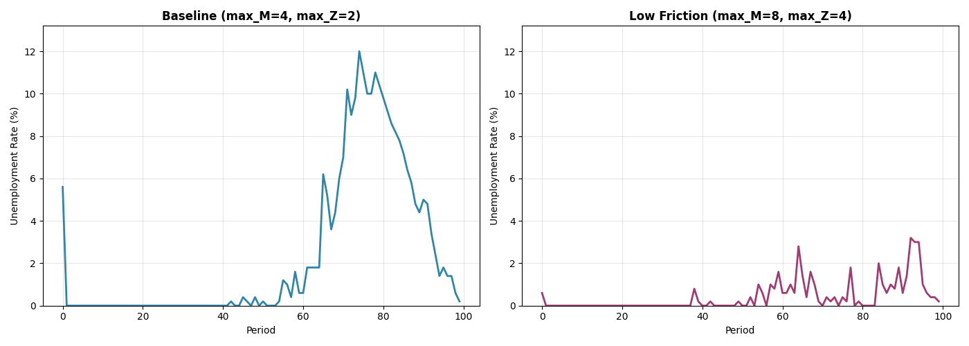
Visualize Comparison

Compare unemployment rates between scenarios.

import matplotlib.pyplot as plt

# Calculate unemployment rates from Worker.employed data
baseline_employed = baseline_results["Worker.employed"]
lowfric_employed = lowfric_results["Worker.employed"]

baseline_unemp = calc_unemployment(baseline_employed) * 100
lowfric_unemp = calc_unemployment(lowfric_employed) * 100

fig, (ax1, ax2) = plt.subplots(1, 2, figsize=(14, 5))

# Calculate y-axis limit
y_max = max(baseline_unemp.max(), lowfric_unemp.max()) * 1.1
y_max = max(y_max, 10)  # Ensure minimum visible range

# Baseline
ax1.plot(baseline_unemp, linewidth=2, color="#2E86AB")
ax1.set_title("Baseline (max_M=4, max_Z=2)", fontsize=12, fontweight="bold")
ax1.set_xlabel("Period")
ax1.set_ylabel("Unemployment Rate (%)")
ax1.grid(True, alpha=0.3)
ax1.set_ylim([0, y_max])

# Low friction
ax2.plot(lowfric_unemp, linewidth=2, color="#A23B72")
ax2.set_title("Low Friction (max_M=8, max_Z=4)", fontsize=12, fontweight="bold")
ax2.set_xlabel("Period")
ax2.set_ylabel("Unemployment Rate (%)")
ax2.grid(True, alpha=0.3)
ax2.set_ylim([0, y_max])

plt.tight_layout()
plt.show()

Summary Statistics

Compare key metrics between scenarios.

print("\n" + "=" * 60)
print("COMPARISON: Baseline vs Low Friction")
print("=" * 60)
print("\nAverage Unemployment Rate:")
print(f"  Baseline (max_M=4, max_Z=2):     {baseline_unemp[20:].mean():.2f}%")
print(f"  Low Friction (max_M=8, max_Z=4): {lowfric_unemp[20:].mean():.2f}%")

baseline_price = sim_baseline.ec.avg_mkt_price
lowfric_price = sim_low_friction_run.ec.avg_mkt_price
print("\nFinal Average Price:")
print(f"  Baseline (max_M=4, max_Z=2):     {baseline_price:.2f}")
print(f"  Low Friction (max_M=8, max_Z=4): {lowfric_price:.2f}")
print("=" * 60)

============================================================
COMPARISON: Baseline vs Low Friction
============================================================

Average Unemployment Rate:
  Baseline (max_M=4, max_Z=2):     2.93%
  Low Friction (max_M=8, max_Z=4): 0.52%

Final Average Price:
  Baseline (max_M=4, max_Z=2):     0.73
  Low Friction (max_M=8, max_Z=4): 1.04
============================================================

Available Parameters

For a complete list of configurable parameters, see the package defaults file or the API documentation.

Common parameters include:

Agent counts:

• n_firms, n_households, n_banks

Shock widths (uniform random ±):

• h_rho (production), h_xi (wage), h_phi (bank expense), h_eta (price)

Search frictions:

• max_M (job applications), max_H (loan applications), max_Z (shopping rounds)

Structural parameters:

• theta (contract duration), beta (consumption propensity exponent)

• delta (dividend rate), v (bank capital coefficient)

• r_bar (baseline interest rate)

Initial conditions:

• price_init, equity_base_init, savings_init, etc.