Robustness Analysis

This example demonstrates robustness analysis inspired by Section 3.10 of Macroeconomics from the Bottom-up (Delli Gatti et al., 2011).

The analysis uses the Growth+ model (with R&D extension for endogenous productivity growth), matching the book’s robustness section. It comprises two parts:

1. Internal validity – run simulations with different random seeds and verify that cross-simulation variance is small and the co-movement structure is stable.

2. Sensitivity analysis – vary one parameter at a time while holding all others at baseline values, checking whether key qualitative results persist.

For the full analysis (20 seeds x 5 experiments x 5-7 values), use:

python -m validation.robustness

This example uses reduced settings for a quick demonstration.

Statistical Helpers

Four pure functions for time series analysis. These are the building blocks of the robustness analysis: the Hodrick-Prescott filter extracts cyclical components from trending series, cross-correlation measures lead-lag structure, and the AR model + impulse-response characterize persistence.

import numpy as np
from scipy import sparse
from scipy.sparse.linalg import spsolve


def hp_filter(y, lamb=1600.0):
    """Hodrick-Prescott filter: decompose *y* into trend + cycle.

    Solves min_tau  sum(y - tau)^2 + lamb * sum(delta^2 tau)^2
    via the sparse linear system (I + lamb * K'K) tau = y.
    """
    t = len(y)
    if t < 3:
        return y.copy(), np.zeros_like(y)
    diags = np.array([np.ones(t - 2), -2 * np.ones(t - 2), np.ones(t - 2)])
    k_mat = sparse.diags(diags, [0, 1, 2], shape=(t - 2, t), format="csc")
    identity = sparse.eye(t, format="csc")
    trend = spsolve(identity + lamb * (k_mat.T @ k_mat), y)
    return trend, y - trend


def cross_correlation(x, y, max_lag=4):
    """Cross-correlation of *x* and *y* at lags ``-max_lag`` to ``+max_lag``."""
    n = len(x)
    result = np.zeros(2 * max_lag + 1)
    for k in range(-max_lag, max_lag + 1):
        if k >= 0:
            x_seg, y_seg = x[: n - k], y[k:]
        else:
            x_seg, y_seg = x[-k:], y[: n + k]
        if len(x_seg) >= 3:
            result[max_lag + k] = np.corrcoef(x_seg, y_seg)[0, 1]
        else:
            result[max_lag + k] = np.nan
    return result


def fit_ar(y, order=2):
    """Fit an AR(*p*) model via OLS.  Returns ``(coeffs, R_squared)``."""
    t = len(y)
    x_mat = np.ones((t - order, order + 1))
    for lag in range(1, order + 1):
        x_mat[:, lag] = y[order - lag : t - lag]
    y_dep = y[order:]
    coeffs, _, _, _ = np.linalg.lstsq(x_mat, y_dep, rcond=None)
    y_pred = x_mat @ coeffs
    ss_res = np.sum((y_dep - y_pred) ** 2)
    ss_tot = np.sum((y_dep - np.mean(y_dep)) ** 2)
    return coeffs, float(1.0 - ss_res / ss_tot if ss_tot > 0 else 0.0)


def impulse_response(ar_coeffs, n_periods=20):
    """Impulse-response function from AR coefficients (unit shock at t=0)."""
    phi = ar_coeffs[1:]  # skip constant
    irf = np.zeros(n_periods)
    irf[0] = 1.0
    for t in range(1, n_periods):
        for lag in range(min(t, len(phi))):
            irf[t] += phi[lag] * irf[t - lag - 1]
    return irf

Growth+ Extension (R&D)

The book’s robustness analysis (Section 3.10) uses the Growth+ model with endogenous productivity growth from R&D investment. We define the extension inline: one custom role tracking R&D state, and three events implementing the R&D mechanism from Equation 3.15.

import bamengine as bam
from bamengine import Float, event, ops, role


@role
class RnD:
    """R&D state for Growth+ extension."""

    sigma: Float  # R&D share of profits
    rnd_intensity: Float  # Expected productivity gain (mu)
    productivity_increment: Float  # Actual productivity increment (z)
    fragility: Float  # Financial fragility (wage_bill / net_worth)


@event(name="firms_compute_rnd_intensity", after="firms_validate_debt_commitments")
class FirmsComputeRnDIntensity:
    """Compute R&D share and intensity for firms."""

    def execute(self, sim):
        bor = sim.get_role("Borrower")
        prod = sim.get_role("Producer")
        emp = sim.get_role("Employer")
        rnd = sim.get_role("RnD")

        eps = 1e-10
        safe_nw = ops.where(ops.greater(bor.net_worth, eps), bor.net_worth, eps)
        fragility = ops.divide(emp.wage_bill, safe_nw)
        ops.assign(rnd.fragility, fragility)

        decay = ops.exp(ops.multiply(sim.sigma_decay, fragility))
        sigma = ops.add(
            sim.sigma_min, ops.multiply(sim.sigma_max - sim.sigma_min, decay)
        )
        sigma = ops.where(ops.greater(bor.net_profit, 0.0), sigma, 0.0)
        ops.assign(rnd.sigma, sigma)

        revenue = ops.multiply(prod.price, prod.production)
        safe_rev = ops.where(ops.greater(revenue, eps), revenue, eps)
        mu = ops.divide(ops.multiply(sigma, bor.net_profit), safe_rev)
        mu = ops.where(ops.greater(mu, 0.0), mu, 0.0)
        ops.assign(rnd.rnd_intensity, mu)


@event(after="firms_compute_rnd_intensity")
class FirmsApplyProductivityGrowth:
    """Apply productivity growth based on R&D."""

    def execute(self, sim):
        prod = sim.get_role("Producer")
        rnd = sim.get_role("RnD")

        z = ops.zeros(sim.n_firms)
        active = ops.greater(rnd.rnd_intensity, 0.0)
        if ops.any(active):
            z[active] = sim.rng.exponential(scale=rnd.rnd_intensity[active])

        ops.assign(rnd.productivity_increment, z)
        ops.assign(prod.labor_productivity, ops.add(prod.labor_productivity, z))


@event(after="firms_apply_productivity_growth")
class FirmsDeductRnDExpenditure:
    """Adjust net profit for R&D expenditure."""

    def execute(self, sim):
        bor = sim.get_role("Borrower")
        rnd = sim.get_role("RnD")
        new_net_profit = ops.multiply(bor.net_profit, ops.subtract(1.0, rnd.sigma))
        ops.assign(bor.net_profit, new_net_profit)


RND_EVENTS = [
    FirmsComputeRnDIntensity,
    FirmsApplyProductivityGrowth,
    FirmsDeductRnDExpenditure,
]

RND_CONFIG = {
    "sigma_min": 0.0,
    "sigma_max": 0.1,
    "sigma_decay": -1.0,
}

Run Multiple Seeds

Internal validity runs the same model with different random seeds. If the model is robust, cross-simulation variance should be small and the co-movement structure should be stable.

N_SEEDS = 3
N_PERIODS = 200
BURN_IN = 100
MAX_LAG = 4

COLLECT_CONFIG = {
    "Producer": ["production", "labor_productivity"],
    "Worker": ["wage", "employed"],
    "Employer": ["n_vacancies"],
    "capture_timing": {
        # Capture wages after workers receive them (not stale previous-period value)
        "Worker.wage": "workers_receive_wage",
        # Capture employment after production (steady-state, before bankruptcy resets)
        "Worker.employed": "firms_run_production",
        # Capture production after it happens
        "Producer.production": "firms_run_production",
        # Capture productivity after R&D growth is applied (captures the increment)
        "Producer.labor_productivity": "firms_apply_productivity_growth",
        # Capture vacancies right after firms decide them
        "Employer.n_vacancies": "firms_decide_vacancies",
    },
}

# The four co-movement variables we track against GDP
COMOVEMENT_VARS = ["unemployment", "productivity", "price_index", "real_wage"]

VARIABLE_TITLES = {
    "unemployment": "Unemployment",
    "productivity": "Productivity",
    "price_index": "Price index",
    "real_wage": "Real wage",
}


def setup_growth_plus(sim):
    """Attach R&D extension to a simulation."""
    sim.use_role(RnD)
    sim.use_events(*RND_EVENTS)
    sim.use_config(RND_CONFIG)


def extract_series(results, n_periods):
    """Extract macro time series from simulation results."""
    production = results.get("Producer", "production")
    productivity = results.get("Producer", "labor_productivity")
    wages = results.get("Worker", "wage")
    employed = results.get("Worker", "employed")
    avg_price = results["Economy.avg_price"]
    inflation = results["Economy.inflation"]

    gdp = ops.sum(production, axis=1)
    unemployment = 1 - ops.mean(employed.astype(float), axis=1)
    log_gdp = ops.log(gdp + 1e-10)

    # Production-weighted average productivity
    weighted = ops.sum(ops.multiply(productivity, production), axis=1)
    avg_productivity = ops.divide(weighted, gdp)

    # Average wage for employed workers only
    emp_wage_sum = ops.sum(ops.where(employed, wages, 0.0), axis=1)
    emp_count = ops.sum(employed, axis=1)
    avg_wage = ops.where(
        ops.greater(emp_count, 0), ops.divide(emp_wage_sum, emp_count), 0.0
    )
    real_wage = ops.divide(avg_wage, avg_price)

    return {
        "gdp": gdp,
        "log_gdp": log_gdp,
        "unemployment": unemployment,
        "productivity": avg_productivity,
        "price_index": avg_price,
        "real_wage": real_wage,
        "inflation": inflation,
    }


def compute_comovements(series, burn_in, max_lag=4):
    """HP-filter GDP and each variable, then compute cross-correlations."""
    _, gdp_cycle = hp_filter(series["log_gdp"][burn_in:])
    comovements = {}
    for var in COMOVEMENT_VARS:
        _, var_cycle = hp_filter(series[var][burn_in:])
        comovements[var] = cross_correlation(gdp_cycle, var_cycle, max_lag)
    return comovements, gdp_cycle


print(f"Running Growth+ model: {N_SEEDS} seeds, {N_PERIODS} periods each...")

all_comovements = {var: [] for var in COMOVEMENT_VARS}
all_ar_coeffs = []
all_gdp_cycles = []
all_stats = {"unemployment": [], "inflation": [], "gdp_growth": []}
baseline_comovements = {}
baseline_ar_coeffs = None
baseline_irf = None

for seed in range(N_SEEDS):
    sim = bam.Simulation.init(seed=seed)
    setup_growth_plus(sim)
    results = sim.run(collect=COLLECT_CONFIG)

    series = extract_series(results, N_PERIODS)
    comovements, gdp_cycle = compute_comovements(series, BURN_IN, MAX_LAG)

    # Collect per-seed co-movements and GDP cycles
    for var in COMOVEMENT_VARS:
        all_comovements[var].append(comovements[var])
    all_gdp_cycles.append(gdp_cycle)
    if seed == 0:
        baseline_comovements = comovements

    # AR fit on GDP cyclical component
    ar_coeffs, ar_r2 = fit_ar(gdp_cycle, order=2)
    all_ar_coeffs.append(ar_coeffs)
    if seed == 0:
        baseline_ar_coeffs = ar_coeffs
        baseline_irf = impulse_response(ar_coeffs, n_periods=20)

    # Cross-simulation statistics
    bi = BURN_IN
    all_stats["unemployment"].append(np.mean(series["unemployment"][bi:]))
    all_stats["inflation"].append(np.mean(series["inflation"][bi:]))
    gdp_gr = np.diff(series["gdp"][bi:]) / series["gdp"][bi:-1]
    all_stats["gdp_growth"].append(np.mean(gdp_gr))

    u = np.mean(series["unemployment"][bi:])
    print(f"  Seed {seed}: unemployment={u:.1%}, AR R\u00b2={ar_r2:.2f}")

Running Growth+ model: 3 seeds, 200 periods each...
  Seed 0: unemployment=9.1%, AR R²=0.60
  Seed 1: unemployment=8.8%, AR R²=0.56
  Seed 2: unemployment=8.4%, AR R²=0.66

Cross-Simulation Summary

A robust model should show small cross-simulation variance: different random seeds produce quantitatively similar results. The coefficient of variation (CV = std/mean) summarizes relative dispersion.

print(f"\nCross-Simulation Variance ({N_SEEDS} seeds):")
print(f"{'Statistic':<25} {'Mean':>10} {'Std':>10} {'CV':>10}")
print("-" * 57)
for name, values in all_stats.items():
    arr = np.array(values)
    mean, std = np.mean(arr), np.std(arr)
    cv = std / abs(mean) if abs(mean) > 1e-10 else float("inf")
    print(f"{name:<25} {mean:>10.4f} {std:>10.4f} {cv:>10.3f}")

# Mean co-movements across seeds
mean_comovements = {}
for var in COMOVEMENT_VARS:
    mean_comovements[var] = np.mean(all_comovements[var], axis=0)

print("\nContemporaneous co-movements (lag=0):")
print(f"{'Variable':<20} {'Baseline':>10} {'Mean':>10} {'Std':>10} {'Peak lag':>10}")
print("-" * 62)
for var in COMOVEMENT_VARS:
    base_val = baseline_comovements[var][MAX_LAG]
    mean_val = mean_comovements[var][MAX_LAG]
    std_val = np.std([c[MAX_LAG] for c in all_comovements[var]])
    # Peak lag: lag of max |correlation| in the mean co-movement
    peak_idx = int(np.argmax(np.abs(mean_comovements[var])))
    peak_lag = peak_idx - MAX_LAG
    print(
        f"{var:<20} {base_val:>10.3f} {mean_val:>10.3f}"
        f" {std_val:>10.3f} {peak_lag:>+10d}"
    )

# Firm size kurtosis (from final period of seed 0)
from scipy import stats as sp_stats

sim0 = bam.Simulation.init(seed=0)
setup_growth_plus(sim0)
res0 = sim0.run(collect=COLLECT_CONFIG)
prod0 = res0.get("Producer", "production")[-1]
prod0_pos = prod0[prod0 > 0]
if len(prod0_pos) > 3:
    kurt = sp_stats.kurtosis(prod0_pos)
    print(f"\nFirm size kurtosis (seed 0, sales): {kurt:.2f} (excess; 0 = normal)")

Cross-Simulation Variance (3 seeds):
Statistic                       Mean        Std         CV
---------------------------------------------------------
unemployment                  0.0875     0.0028      0.032
inflation                    -0.0049     0.0004      0.074
gdp_growth                    0.0026     0.0000      0.016

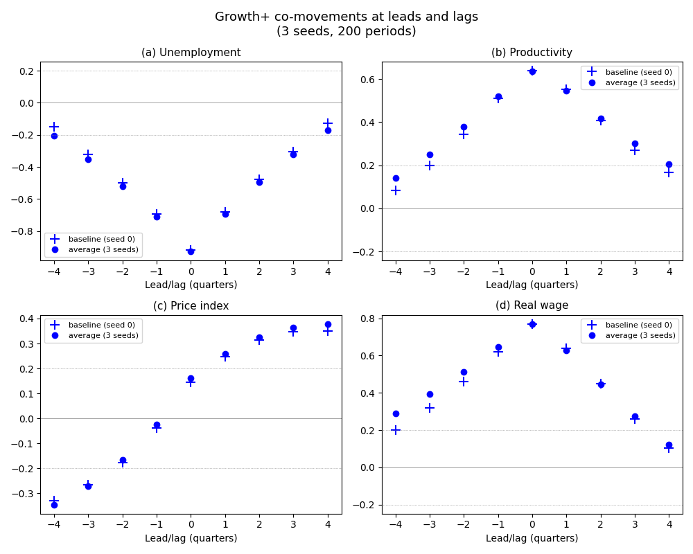
Contemporaneous co-movements (lag=0):
Variable               Baseline       Mean        Std   Peak lag
--------------------------------------------------------------
unemployment             -0.918     -0.927      0.010         +0
productivity              0.638      0.637      0.013         +0
price_index               0.144      0.163      0.018         +4
real_wage                 0.768      0.769      0.005         +0

Firm size kurtosis (seed 0, sales): 68.76 (excess; 0 = normal)

Plot Co-Movements (Figure 3.9)

The co-movement plot is the key output of the internal validity analysis. It shows cross-correlations between HP-filtered GDP and four macro variables at leads and lags from -4 to +4. The baseline (seed 0) is shown as ‘+’ markers; the cross-simulation mean as ‘o’ markers. Dashed lines at +/-0.2 mark the acyclicality band.

import matplotlib.pyplot as plt

PANEL_LABELS = ["(a)", "(b)", "(c)", "(d)"]
lags = np.arange(-MAX_LAG, MAX_LAG + 1)

fig, axes = plt.subplots(2, 2, figsize=(10, 8))
fig.suptitle(
    f"Growth+ co-movements at leads and lags\n({N_SEEDS} seeds, {N_PERIODS} periods)",
    fontsize=13,
    y=0.98,
)

for i, var in enumerate(COMOVEMENT_VARS):
    ax = axes.flat[i]
    ax.plot(
        lags,
        baseline_comovements[var],
        "+",
        markersize=10,
        color="blue",
        markeredgewidth=1.5,
        label="baseline (seed 0)",
    )
    ax.plot(
        lags,
        mean_comovements[var],
        "o",
        markersize=6,
        color="blue",
        markerfacecolor="blue",
        label=f"average ({N_SEEDS} seeds)",
    )
    ax.axhline(0, color="gray", linewidth=0.5)
    ax.axhline(0.2, color="gray", linewidth=0.5, linestyle=":")
    ax.axhline(-0.2, color="gray", linewidth=0.5, linestyle=":")
    ax.set_title(f"{PANEL_LABELS[i]} {VARIABLE_TITLES[var]}", fontsize=11)
    ax.set_xlabel("Lead/lag (quarters)")
    ax.set_xticks(lags)
    ax.legend(fontsize=8, loc="best")

plt.tight_layout()
plt.show()

AR Structure and Impulse Response

Individual seeds are well-described by an AR(2) process with a hump-shaped impulse response (peak at period 1-2, decay to zero by ~10 periods). When we average AR coefficients across seeds, the result is AR(1)-like with monotone exponential decay – the second-order dynamics cancel out.

# Fit AR(1) on the pointwise-averaged GDP cycle across seeds
min_len = min(len(c) for c in all_gdp_cycles)
stacked_cycles = np.array([c[:min_len] for c in all_gdp_cycles])
mean_cycle = np.mean(stacked_cycles, axis=0)
mean_ar1_coeffs, mean_ar1_r2 = fit_ar(mean_cycle, order=1)
mean_irf = impulse_response(mean_ar1_coeffs, n_periods=20)

print("AR Structure:")
print(
    f"  Baseline (seed 0): AR(2), "
    f"phi_1={baseline_ar_coeffs[1]:.3f}, phi_2={baseline_ar_coeffs[2]:.3f}"
)
print(
    f"  Cross-sim mean:    AR(1), "
    f"phi_1={mean_ar1_coeffs[1]:.3f}, R\u00b2={mean_ar1_r2:.3f}"
    f" (fitted on averaged cycle)"
)

fig, ax = plt.subplots(1, 1, figsize=(8, 5))
periods_irf = np.arange(len(baseline_irf))
ax.plot(periods_irf, baseline_irf, "b--", linewidth=1.5, label="Baseline AR(2)")
ax.plot(
    periods_irf,
    mean_irf,
    "b-",
    linewidth=2,
    label=f"Mean AR(1) (\u03c6={mean_ar1_coeffs[1]:.2f})",
)
ax.axhline(0, color="gray", linewidth=0.5)
ax.set_title("GDP cyclical component: impulse-response function", fontsize=12)
ax.set_xlabel("Periods after shock")
ax.set_ylabel("Response")
ax.legend(fontsize=9)
ax.grid(True, alpha=0.3)

plt.tight_layout()
plt.show()

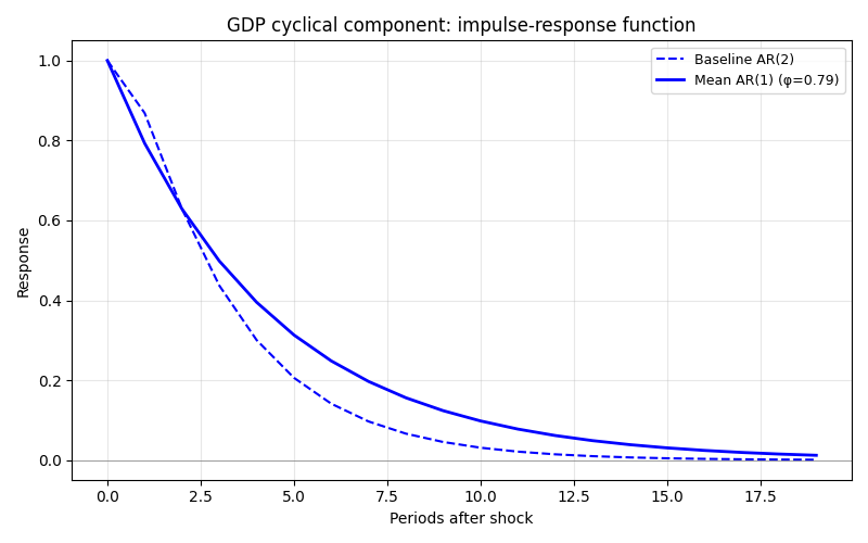
AR Structure:
  Baseline (seed 0): AR(2), phi_1=0.869, phi_2=-0.126
  Cross-sim mean:    AR(1), phi_1=0.793, R²=0.628 (fitted on averaged cycle)

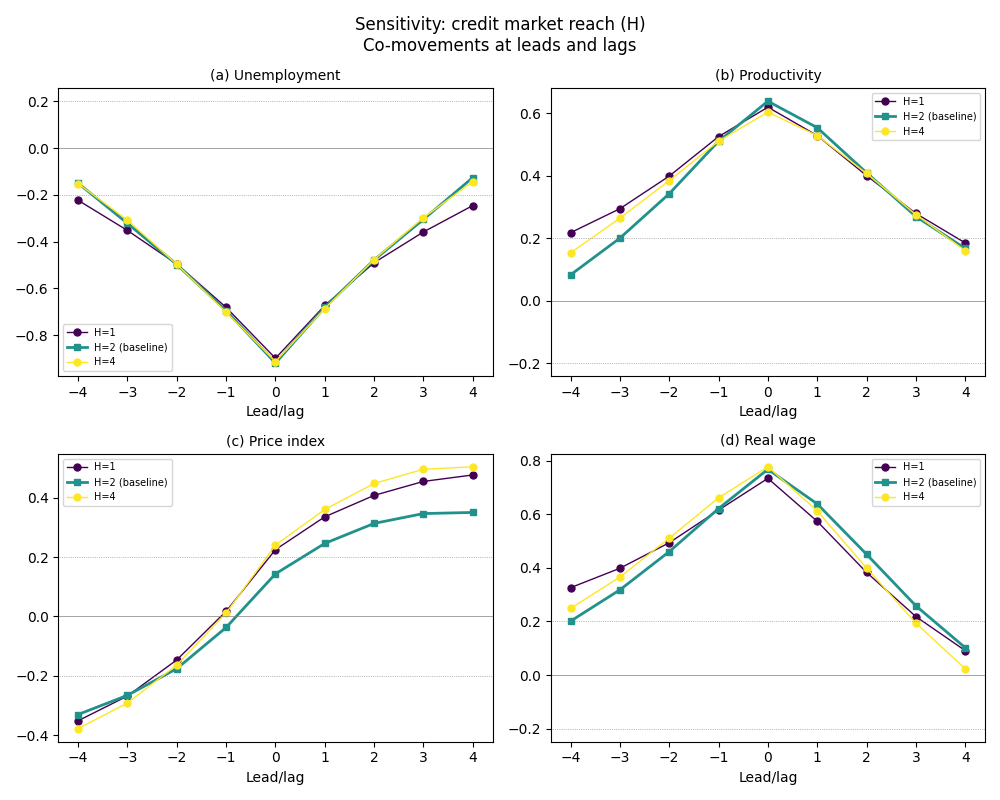
Sensitivity Analysis

Sensitivity analysis varies one parameter at a time. Here we vary H, the number of banks each firm can contact when seeking credit (the “local credit market” parameter from Section 3.10.1(i)). General macro properties should be stable across all H values.

SENSITIVITY_CONFIGS = {
    "H=1": {"max_H": 1},
    "H=2 (baseline)": {},
    "H=4": {"max_H": 4},
}

print("\nSensitivity: varying H (credit market reach)")
print(f"{'Value':<20} {'Unemployment':>15} {'Inflation':>12}")
print("-" * 49)

sensitivity_comovements = {}
for label, overrides in SENSITIVITY_CONFIGS.items():
    sim = bam.Simulation.init(seed=0, **overrides)
    setup_growth_plus(sim)
    results = sim.run(collect=COLLECT_CONFIG)

    series = extract_series(results, N_PERIODS)
    comovements, _ = compute_comovements(series, BURN_IN, MAX_LAG)
    sensitivity_comovements[label] = comovements

    u = np.mean(series["unemployment"][BURN_IN:])
    inf = np.mean(series["inflation"][BURN_IN:])
    print(f"{label:<20} {u:>14.1%} {inf:>11.1%}")

Sensitivity: varying H (credit market reach)
Value                   Unemployment    Inflation
-------------------------------------------------
H=1                            8.1%       -0.5%
H=2 (baseline)                 9.1%       -0.4%
H=4                            9.4%       -0.5%

Plot Sensitivity Co-Movements

Co-movement comparison across parameter values shows how the cyclical structure changes (or stays stable) with parameter variation. The credit market parameter H should preserve the overall structure.

colors = plt.cm.viridis(np.linspace(0, 1, len(SENSITIVITY_CONFIGS)))

fig, axes = plt.subplots(2, 2, figsize=(10, 8))
fig.suptitle(
    "Sensitivity: credit market reach (H)\nCo-movements at leads and lags",
    fontsize=12,
    y=0.98,
)

for i, var in enumerate(COMOVEMENT_VARS):
    ax = axes.flat[i]
    for j, (label, comovs) in enumerate(sensitivity_comovements.items()):
        marker = "s" if "baseline" in label else "o"
        lw = 2.0 if "baseline" in label else 1.0
        ax.plot(
            lags,
            comovs[var],
            marker=marker,
            markersize=5,
            color=colors[j],
            linewidth=lw,
            label=label,
        )
    ax.axhline(0, color="gray", linewidth=0.5)
    ax.axhline(0.2, color="gray", linewidth=0.5, linestyle=":")
    ax.axhline(-0.2, color="gray", linewidth=0.5, linestyle=":")
    ax.set_title(f"{PANEL_LABELS[i]} {VARIABLE_TITLES[var]}", fontsize=10)
    ax.set_xlabel("Lead/lag")
    ax.set_xticks(lags)
    ax.legend(fontsize=7, loc="best")

plt.tight_layout()
plt.show()

Structural Experiments (Section 3.10.2)

Section 3.10.2 describes two experiments that test model mechanisms:

1. PA experiment: Disable consumer loyalty (“preferential attachment”) to show that volatility drops and deep crises vanish.

2. Entry neutrality: Apply heavy profit taxation without redistribution to confirm that automatic firm entry does NOT drive recovery.

Here we run these as simple inline experiments using only bamengine and extensions APIs, reusing the helpers defined above.

PA Experiment (quick demo)

Disabling consumer loyalty removes the positive feedback loop where successful firms attract more customers. Without PA, the economy becomes more “competitive” and less prone to large fluctuations. We compare two runs at the same seed: PA on (default loyalty matching) vs PA off (random matching).

PA_SEED = 0
PA_PERIODS = 200
PA_BURN_IN = 100

print("\n--- PA Experiment (quick demo) ---")

# PA on (default: consumer_matching="loyalty")
sim_on = bam.Simulation.init(seed=PA_SEED)
setup_growth_plus(sim_on)
res_on = sim_on.run(n_periods=PA_PERIODS, collect=COLLECT_CONFIG)
series_on = extract_series(res_on, PA_PERIODS)

# PA off (random matching)
sim_off = bam.Simulation.init(seed=PA_SEED, consumer_matching="random")
setup_growth_plus(sim_off)
res_off = sim_off.run(n_periods=PA_PERIODS, collect=COLLECT_CONFIG)
series_off = extract_series(res_off, PA_PERIODS)

# Compare GDP volatility and AR persistence
bi = PA_BURN_IN
gdp_gr_on = np.diff(series_on["gdp"][bi:]) / series_on["gdp"][bi:-1]
gdp_gr_off = np.diff(series_off["gdp"][bi:]) / series_off["gdp"][bi:-1]
vol_on = np.std(gdp_gr_on)
vol_off = np.std(gdp_gr_off)

_, cycle_on = hp_filter(series_on["log_gdp"][bi:])
_, cycle_off = hp_filter(series_off["log_gdp"][bi:])
ar_on, _ = fit_ar(cycle_on, order=2)
ar_off, _ = fit_ar(cycle_off, order=2)

print(f"  GDP volatility: PA on = {vol_on:.4f}, PA off = {vol_off:.4f}")
print(f"  AR persistence: PA on phi_1 = {ar_on[1]:.3f}, PA off phi_1 = {ar_off[1]:.3f}")

# Plot log GDP time series overlay (post burn-in)
log_gdp_on = series_on["log_gdp"][bi:]
log_gdp_off = series_off["log_gdp"][bi:]
fig, ax = plt.subplots(1, 1, figsize=(12, 5))
periods = np.arange(len(log_gdp_on))
ax.plot(periods, log_gdp_on, "b-", linewidth=1, alpha=0.8, label="PA on (loyalty)")
ax.plot(periods, log_gdp_off, "r-", linewidth=1, alpha=0.8, label="PA off (random)")
ax.set_title("Log GDP: PA on vs PA off (Section 3.10.2, Figure 3.10)", fontsize=12)
ax.set_xlabel("Period (after burn-in)")
ax.set_ylabel("Log GDP")
ax.legend(fontsize=9)
ax.grid(True, alpha=0.3)
plt.tight_layout()
plt.show()

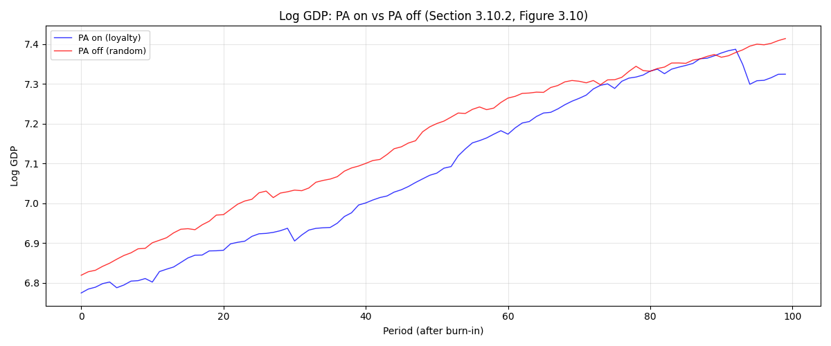
--- PA Experiment (quick demo) ---
  GDP volatility: PA on = 0.0104, PA off = 0.0062
  AR persistence: PA on phi_1 = 0.879, PA off phi_1 = 0.719

Entry Neutrality Experiment (quick demo)

Heavy taxation without redistribution increases bankruptcies. If entry were artificially driving recovery, performance would be unchanged. Instead, we expect monotonic degradation.

from extensions.taxation import TAXATION_CONFIG, TAXATION_EVENTS

ENTRY_SEED = 0
ENTRY_PERIODS = 200
ENTRY_BURN_IN = 100
TAX_RATES = [0.0, 0.5, 0.9]

print("\n--- Entry Neutrality Experiment (quick demo) ---")
print(f"{'Tax rate':<12} {'Unemployment':>15}")
print("-" * 29)

entry_unemployment = []
for tax_rate in TAX_RATES:
    sim = bam.Simulation.init(seed=ENTRY_SEED)
    setup_growth_plus(sim)
    sim.use_events(*TAXATION_EVENTS)
    sim.use_config({**TAXATION_CONFIG, "profit_tax_rate": tax_rate})
    results = sim.run(n_periods=ENTRY_PERIODS, collect=COLLECT_CONFIG)

    series = extract_series(results, ENTRY_PERIODS)
    u_mean = np.mean(series["unemployment"][ENTRY_BURN_IN:])
    entry_unemployment.append(u_mean)
    print(f"{tax_rate:<12.0%} {u_mean:>14.1%}")

# Bar chart showing monotonic degradation
fig, ax = plt.subplots(1, 1, figsize=(6, 4))
labels = [f"{r:.0%}" for r in TAX_RATES]
ax.bar(labels, [u * 100 for u in entry_unemployment], color="steelblue", width=0.5)
ax.set_xlabel("Profit tax rate")
ax.set_ylabel("Mean unemployment (%)")
ax.set_title("Entry neutrality: unemployment vs profit tax rate", fontsize=11)
ax.grid(True, alpha=0.3, axis="y")
plt.tight_layout()
plt.show()

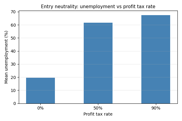
--- Entry Neutrality Experiment (quick demo) ---
Tax rate        Unemployment
-----------------------------
0%                    19.6%
50%                   61.5%
90%                   67.4%