YAML Configuration

This example demonstrates how to configure BAM Engine simulations using YAML files. YAML configuration is useful for:

• Saving and sharing simulation setups

• Running reproducible experiments

• Separating configuration from code

If you’re new to YAML, start with keyword arguments instead (see example_configuration.py).

Creating a Configuration File

Configuration files use YAML format. Here’s an example showing the structure and available parameters.

import tempfile
from pathlib import Path

import numpy as np

import bamengine as bam

# Create a sample config file programmatically
# (normally you'd create this file manually in your editor)
config_content = """
# ==============================================================================
# Sample BAM Engine Configuration
# ==============================================================================

# Population sizes
n_firms: 80
n_households: 400
n_banks: 8

# Stochastic shock parameters (0 = no shocks, higher = more volatility)
h_rho: 0.08      # Production growth shock cap
h_xi: 0.04       # Wage growth shock cap
h_phi: 0.08      # Bank expense shock cap
h_eta: 0.08      # Price adjustment shock cap

# Search frictions (how many partners agents can contact per period)
max_M: 3         # Job applications per unemployed worker
max_H: 2         # Loan applications per firm
max_Z: 3         # Shops per household

# Structural parameters
theta: 10        # Base contract length (periods)
beta: 2.0        # Consumption propensity exponent
delta: 0.35      # Dividend payout ratio
v: 0.08          # Bank capital requirement

# Initial conditions
net_worth_init: 15.0     # Firm initial net worth
price_init: 1.0          # Initial price level
savings_init: 4.0        # Household initial savings
wage_offer_init: 0.85    # Initial wage offer
equity_base_init: 6.0    # Bank initial equity

# Random seed for reproducibility
seed: 42

# Logging configuration
logging:
  default_level:    ERROR
"""

# Write to a temporary file
config_dir = Path(tempfile.mkdtemp())
config_path = config_dir / "my_config.yml"
config_path.write_text(config_content)

print(f"Created config file at: {config_path}")

Created config file at: /tmp/tmpdx5spbyw/my_config.yml

Loading Configuration from YAML

Pass the config file path to Simulation.init().

sim = bam.Simulation.init(config=str(config_path))

print("Loaded configuration:")
print(f"  Firms: {sim.n_firms}")
print(f"  Households: {sim.n_households}")
print(f"  Banks: {sim.n_banks}")

# Run a short simulation to verify it works
sim.run(n_periods=20)
print(f"\nSimulation completed! Final unemployment: {np.mean(~sim.wrk.employed):.2%}")

Loaded configuration:
  Firms: 80
  Households: 400
  Banks: 8

Simulation completed! Final unemployment: 94.25%

Configuration Precedence

BAM Engine uses a three-tier precedence system:

1. Package defaults (config/defaults.yml)

2. User config file (your YAML)

3. Keyword arguments (highest priority)

Keyword arguments always override YAML values.

# Override specific values from YAML
sim_override = bam.Simulation.init(
    config=str(config_path),
    n_firms=150,  # Override YAML's n_firms=80
    seed=999,  # Override YAML's seed=42
)

print("With kwargs override:")
print(f"  Firms: {sim_override.n_firms}")  # 150 (from kwargs)
print(f"  Households: {sim_override.n_households}")  # 400 (from YAML)

With kwargs override:
  Firms: 150
  Households: 400

Using a Dictionary as Config

Instead of a file path, you can pass a dictionary directly. This is useful for programmatic configuration or quick experiments.

config_dict = {
    "n_firms": 120,
    "n_households": 600,
    "n_banks": 12,
    "h_rho": 0.05,  # Lower shocks for stability
    "theta": 12,  # Longer contracts
    "seed": 12345,
}

sim_dict = bam.Simulation.init(config=config_dict)

print("From dictionary config:")
print(f"  Firms: {sim_dict.n_firms}")
print(f"  Households: {sim_dict.n_households}")
print(f"  Shock cap (h_rho): {sim_dict.config.h_rho}")

From dictionary config:
  Firms: 120
  Households: 600
  Shock cap (h_rho): 0.05

Comparing Different Configurations

Run two scenarios with different configurations and compare results.

import matplotlib.pyplot as plt

# Scenario 1: High friction economy (fewer search attempts)
high_friction_config = {
    "n_firms": 100,
    "n_households": 500,
    "max_M": 2,  # Fewer job applications
    "max_H": 1,  # Fewer loan applications
    "max_Z": 1,  # Fewer shopping rounds
    "seed": 42,
}

# Scenario 2: Low friction economy (more search attempts)
low_friction_config = {
    "n_firms": 100,
    "n_households": 500,
    "max_M": 6,  # More job applications
    "max_H": 4,  # More loan applications
    "max_Z": 4,  # More shopping rounds
    "seed": 42,
}

# Run both simulations with data collection for unemployment calculation
n_periods = 100

# High friction simulation
sim_high = bam.Simulation.init(config=high_friction_config)
wrk_high = sim_high.get_role("Worker")
unemployment_high = []
for _ in range(n_periods):
    sim_high.step()
    # Calculate unemployment from Worker.employed (preferred method)
    unemp = 1.0 - bam.ops.mean(wrk_high.employed.astype(float))
    unemployment_high.append(unemp * 100)

# Low friction simulation
sim_low = bam.Simulation.init(config=low_friction_config)
wrk_low = sim_low.get_role("Worker")
unemployment_low = []
for _ in range(n_periods):
    sim_low.step()
    unemp = 1.0 - bam.ops.mean(wrk_low.employed.astype(float))
    unemployment_low.append(unemp * 100)

# Convert to arrays for plotting
unemployment_high = bam.ops.asarray(unemployment_high)
unemployment_low = bam.ops.asarray(unemployment_low)

# Compare unemployment rates
fig, ax = plt.subplots(figsize=(10, 6))

ax.plot(unemployment_high, label="High Friction", linewidth=2)
ax.plot(unemployment_low, label="Low Friction", linewidth=2)
ax.set_xlabel("Period")
ax.set_ylabel("Unemployment Rate (%)")
ax.set_title("Effect of Search Frictions on Unemployment")
ax.legend()
ax.grid(True, alpha=0.3)
plt.tight_layout()
plt.show()

# Print summary statistics using ops
print("\nSummary Statistics:")
print(f"{'Scenario':<15} {'Mean Unemp.':<15} {'Std Unemp.':<15}")
print("-" * 45)
print(
    f"{'High Friction':<15} {bam.ops.mean(unemployment_high):>12.2f}% "
    f"{bam.ops.std(unemployment_high):>12.2f}%"
)
print(
    f"{'Low Friction':<15} {bam.ops.mean(unemployment_low):>12.2f}% "
    f"{bam.ops.std(unemployment_low):>12.2f}%"
)

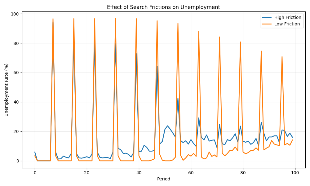
Summary Statistics:
Scenario        Mean Unemp.     Std Unemp.
---------------------------------------------
High Friction          14.86%        18.10%
Low Friction           13.53%        28.33%

Key Configuration Parameters Reference

Here’s a quick reference of the most commonly used parameters:

Population sizes:

• n_firms: Number of producer/employer agents

• n_households: Number of worker/consumer agents

• n_banks: Number of lender agents

Shock parameters (volatility):

• h_rho: Production growth shock magnitude

• h_xi: Wage growth shock magnitude

• h_phi: Bank expense shock magnitude

• h_eta: Price adjustment shock magnitude

Search frictions:

• max_M: Job applications per unemployed worker per period

• max_H: Loan applications per firm per period

• max_Z: Shops a household can visit per period

Structural parameters:

• theta: Base job contract length (periods)

• beta: Consumption propensity exponent

• delta: Dividend payout ratio

• v: Bank capital requirement

See config/defaults.yml in the package for the complete list.

# Clean up
import shutil

shutil.rmtree(config_dir)
print("\nConfig file cleaned up.")

Config file cleaned up.