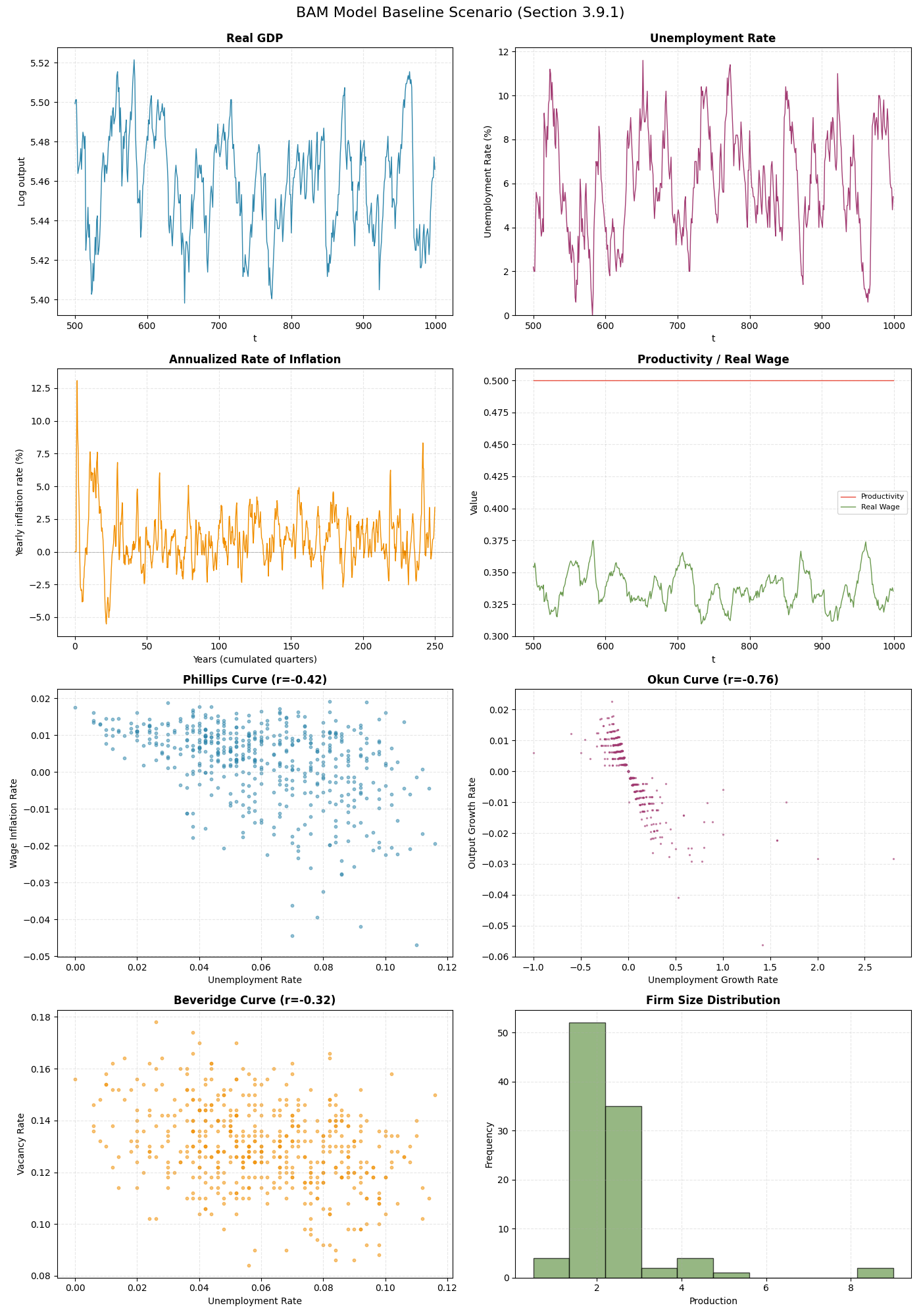
BAM Baseline Scenario

This example reproduces the baseline scenario from section 3.9.1 of the original BAM model book (Delli Gatti et al., 2011). This scenario demonstrates the fundamental dynamics of the model with standard parameter values.

We visualize eight panels: four time series (real GDP, unemployment rate, inflation rate, productivity-real wage) and four macroeconomic curves (Phillips, Okun, Beveridge, and firm size distribution).

For detailed validation with bounds and statistical annotations, run:

python -m validation.scenarios.baseline

Initialize Simulation

Create a simulation using default parameters that correspond to the baseline scenario.

import bamengine as bam
from bamengine import ops

sim = bam.Simulation.init()

print("Initialized baseline scenario with:")
print(f"  - {sim.n_firms} firms")
print(f"  - {sim.n_households} households")
print(f"  - {sim.n_banks} banks")

Initialized baseline scenario with:
  - 100 firms
  - 500 households
  - 10 banks

Run Simulation

Run with data collection for key economic indicators.

COLLECT_CONFIG = {
    "Producer": ["production", "labor_productivity"],
    "Worker": ["wage", "employed"],
    "Employer": ["n_vacancies"],
    "capture_timing": {
        # Capture wages after workers receive them (not stale previous-period value)
        "Worker.wage": "workers_receive_wage",
        # Capture employment after production (steady-state, before bankruptcy resets)
        "Worker.employed": "firms_run_production",
        # Capture production after it happens
        "Producer.production": "firms_run_production",
        # Capture vacancies right after firms decide them
        "Employer.n_vacancies": "firms_decide_vacancies",
    },
}

results = sim.run(collect=COLLECT_CONFIG)

print(f"\nSimulation completed: {results.metadata['n_periods']} periods")
print(f"Runtime: {results.metadata['runtime_seconds']:.2f} seconds")

Simulation completed: 1000 periods
Runtime: 5.44 seconds

Compute Metrics

Compute key economic indicators from the simulation results.

import numpy as np

burn_in = 500
n_periods = sim.n_periods

# Extract raw data from results
avg_price = results["Economy.avg_price"]
production = results.get("Producer", "production")
productivity = results.get("Producer", "labor_productivity")
wages = results.get("Worker", "wage")
employed_arr = results.get("Worker", "employed")
n_vacancies = results.get("Employer", "n_vacancies")

# Compute total production (GDP)
total_production = ops.sum(production, axis=1)

# Unemployment rate (fraction of workers not employed)
unemployment = 1 - ops.mean(employed_arr.astype(float), axis=1)

# Log GDP
log_gdp = ops.log(total_production + 1e-10)

# Annual inflation rate
inflation = results["Economy.inflation"]

# Average wage for employed workers
employed_wages_sum = ops.sum(ops.where(employed_arr, wages, 0.0), axis=1)
employed_count = ops.sum(employed_arr, axis=1)
avg_wage = ops.where(
    ops.greater(employed_count, 0),
    ops.divide(employed_wages_sum, employed_count),
    0.0,
)

# Real wage
real_wage = ops.divide(avg_wage, avg_price)

# Production-weighted average productivity
weighted_prod = ops.sum(ops.multiply(productivity, production), axis=1)
avg_productivity = ops.divide(weighted_prod, total_production)

# Wage inflation for Phillips curve
wage_inflation = ops.divide(
    avg_wage[1:] - avg_wage[:-1],
    ops.where(ops.greater(avg_wage[:-1], 0), avg_wage[:-1], 1.0),
)

# GDP growth for Okun curve
gdp_growth = ops.divide(
    total_production[1:] - total_production[:-1], total_production[:-1]
)

# Unemployment growth for Okun curve
unemployment_growth = ops.divide(
    unemployment[1:] - unemployment[:-1],
    ops.where(ops.greater(unemployment[:-1], 0), unemployment[:-1], 1.0),
)

# Vacancy rate for Beveridge curve
total_vacancies = ops.sum(n_vacancies, axis=1)
vacancy_rate = ops.divide(total_vacancies, sim.n_households)

# Final period firm production
prod = sim.get_role("Producer")
final_production = prod.production.copy()

# Correlations
phillips_corr = np.corrcoef(unemployment[burn_in:], wage_inflation[burn_in - 1 :])[0, 1]
okun_corr = np.corrcoef(unemployment_growth[burn_in - 1 :], gdp_growth[burn_in - 1 :])[
    0, 1
]
beveridge_corr = np.corrcoef(unemployment[burn_in:], vacancy_rate[burn_in:])[0, 1]

print(f"\nKey metrics (after {burn_in}-period burn-in):")
print(f"  Unemployment: {np.mean(unemployment[burn_in:]) * 100:.1f}%")
print(f"  Inflation: {np.mean(inflation[burn_in:]) * 100:.1f}%")
print(f"  Phillips correlation: {phillips_corr:.2f}")
print(f"  Okun correlation: {okun_corr:.2f}")
print(f"  Beveridge correlation: {beveridge_corr:.2f}")

Key metrics (after 500-period burn-in):
  Unemployment: 6.0%
  Inflation: 1.1%
  Phillips correlation: -0.42
  Okun correlation: -0.76
  Beveridge correlation: -0.32

Visualize Results

Create a simple 4x2 figure showing time series and macroeconomic curves.

import matplotlib.pyplot as plt

periods = ops.arange(burn_in, n_periods)
fig, axes = plt.subplots(4, 2, figsize=(14, 20))
fig.suptitle("BAM Model Baseline Scenario (Section 3.9.1)", fontsize=16, y=0.995)

# Panel (0,0): Log Real GDP
ax = axes[0, 0]
ax.plot(periods, log_gdp[burn_in:], linewidth=1, color="#2E86AB")
ax.set_title("Real GDP", fontsize=12, fontweight="bold")
ax.set_ylabel("Log output")
ax.set_xlabel("t")
ax.grid(True, linestyle="--", alpha=0.3)

# Panel (0,1): Unemployment Rate
ax = axes[0, 1]
ax.plot(periods, unemployment[burn_in:] * 100, linewidth=1, color="#A23B72")
ax.set_title("Unemployment Rate", fontsize=12, fontweight="bold")
ax.set_ylabel("Unemployment Rate (%)")
ax.set_xlabel("t")
ax.set_ylim(bottom=0)
ax.grid(True, linestyle="--", alpha=0.3)

# Panel (1,0): Annual Inflation Rate (all periods, x-axis in cumulated years)
ax = axes[1, 0]
years = ops.arange(0, n_periods) / 4
ax.plot(years, inflation * 100, linewidth=1, color="#F18F01")
ax.axhline(0, color="black", linestyle="-", alpha=0.3, linewidth=0.5)
ax.set_title("Annualized Rate of Inflation", fontsize=12, fontweight="bold")
ax.set_ylabel("Yearly inflation rate (%)")
ax.set_xlabel("Years (cumulated quarters)")
ax.grid(True, linestyle="--", alpha=0.3)

# Panel (1,1): Productivity and Real Wage (with legend)
ax = axes[1, 1]
ax.plot(
    periods,
    avg_productivity[burn_in:],
    linewidth=1,
    color="#E74C3C",
    label="Productivity",
)
ax.plot(periods, real_wage[burn_in:], linewidth=1, color="#6A994E", label="Real Wage")
ax.set_title("Productivity / Real Wage", fontsize=12, fontweight="bold")
ax.set_ylabel("Value")
ax.set_xlabel("t")
ax.legend(loc="center right", fontsize=8)
ax.grid(True, linestyle="--", alpha=0.3)

# Panel (2,0): Phillips Curve
ax = axes[2, 0]
ax.scatter(
    unemployment[burn_in:],
    wage_inflation[burn_in - 1 :],
    s=10,
    alpha=0.5,
    color="#2E86AB",
)
ax.set_title(f"Phillips Curve (r={phillips_corr:.2f})", fontsize=12, fontweight="bold")
ax.set_xlabel("Unemployment Rate")
ax.set_ylabel("Wage Inflation Rate")
ax.grid(True, linestyle="--", alpha=0.3)

# Panel (2,1): Okun Curve
ax = axes[2, 1]
ax.scatter(
    unemployment_growth[burn_in - 1 :],
    gdp_growth[burn_in - 1 :],
    s=2,
    alpha=0.5,
    color="#A23B72",
)
ax.set_title(f"Okun Curve (r={okun_corr:.2f})", fontsize=12, fontweight="bold")
ax.set_xlabel("Unemployment Growth Rate")
ax.set_ylabel("Output Growth Rate")
ax.grid(True, linestyle="--", alpha=0.3)

# Panel (3,0): Beveridge Curve
ax = axes[3, 0]
ax.scatter(
    unemployment[burn_in:], vacancy_rate[burn_in:], s=10, alpha=0.5, color="#F18F01"
)
ax.set_title(
    f"Beveridge Curve (r={beveridge_corr:.2f})", fontsize=12, fontweight="bold"
)
ax.set_xlabel("Unemployment Rate")
ax.set_ylabel("Vacancy Rate")
ax.grid(True, linestyle="--", alpha=0.3)

# Panel (3,1): Firm Size Distribution
ax = axes[3, 1]
ax.hist(final_production, bins=10, edgecolor="black", alpha=0.7, color="#6A994E")
ax.set_title("Firm Size Distribution", fontsize=12, fontweight="bold")
ax.set_xlabel("Production")
ax.set_ylabel("Frequency")
ax.grid(True, linestyle="--", alpha=0.3)

plt.tight_layout()
plt.show()