Buffer-Stock Consumption Extension

This example implements the buffer-stock consumption extension from Section 3.9.4 of Macroeconomics from the Bottom-up, replacing the baseline mean-field MPC with an individual adaptive rule based on buffer-stock saving theory.

Key Equations

Buffer-Stock MPC (Equation 3.20):

\[c_t = 1 + \frac{d_t - h \cdot g_t}{1 + g_t}\]

Where: - \(h\) is the desired savings-income ratio - \(g_t = W_t / W_{t-1} - 1\) is the income growth rate - \(d_t = S_t / W_{t-1} - h\) is the divergence from desired ratio

Fresh Start Formula (just re-employed):

\[c_t = 1 - h + S_t / W_t\]

This example demonstrates:

• Defining replacement events with @event(replace=...) to swap pipeline behavior

• How the buffer-stock MPC differs from the baseline mean-field rule

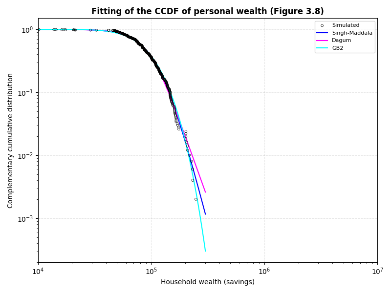
• Fitting heavy-tailed distributions (Singh-Maddala, Dagum, GB2) to wealth data

• CCDF plotting on log-log axes (Figure 3.8 from the book)

For detailed validation with bounds and statistical annotations, run:

python -m validation.scenarios.buffer_stock

Import Dependencies

We import BAM Engine and the decorators needed to define custom components.

import bamengine as bam
from bamengine import Float, event, ops, role
from extensions.rnd import RND_EVENTS, RnD

Define Custom Role: BufferStock

The BufferStock role tracks previous-period income and the computed MPC (propensity) for each household.

@role
class BufferStock:
    """Buffer-stock consumption state for households."""

    prev_income: Float  # W_{t-1}: previous period income
    propensity: Float  # c_t: buffer-stock MPC (may exceed 1.0)

Define Replacement Events

Two events replace the baseline consumption logic. @event(replace=...) removes the original event from the pipeline and inserts the new one in its place.

@event(replace="consumers_calc_propensity")
class ConsumersCalcBufferStockPropensity:
    """Compute individual MPC using buffer-stock adaptive rule.

    Three cases:
    1. Normal (both incomes positive): Full Eq. 3.20
    2. Fresh start (just re-employed): c = 1 - h + S/W
    3. Unemployed (no income): c = 1/h (gradual savings drawdown)
    """

    def execute(self, sim: bam.Simulation) -> None:
        con = sim.get_role("Consumer")
        buf = sim.get_role("BufferStock")

        income = con.income
        prev_income = buf.prev_income
        savings = con.savings
        h = sim.buffer_stock_h

        normal = (prev_income > 0) & (income > 0)
        fresh = (prev_income <= 0) & (income > 0)

        c = ops.full(len(income), 1 / h)  # default: c=1/h (unemployed drawdown)

        if ops.any(normal):
            g = income[normal] / prev_income[normal] - 1.0
            g = ops.maximum(g, -0.99)  # g=-1.0 leads to singularity, so cap at -0.99
            d = savings[normal] / prev_income[normal] - h
            c[normal] = 1.0 + (d - h * g) / (1.0 + g)

        if ops.any(fresh):
            c[fresh] = 1.0 - h + savings[fresh] / income[fresh]

        c = ops.maximum(c, 0.0)
        ops.assign(buf.propensity, c)


@event(replace="consumers_decide_income_to_spend")
class ConsumersDecideBufferStockSpending:
    """Allocate spending budget using buffer-stock MPC.

    Employed: budget = c * income
    Unemployed: budget = c * savings
    """

    def execute(self, sim: bam.Simulation) -> None:
        con = sim.get_role("Consumer")
        buf = sim.get_role("BufferStock")

        c = buf.propensity
        income = con.income
        savings = con.savings

        employed = income > 0
        budget = ops.where(employed, c * income, c * savings)
        budget = ops.minimum(budget, savings + income)
        budget = ops.maximum(budget, 0.0)

        ops.assign(buf.prev_income, income)
        ops.assign(con.income_to_spend, budget)

        new_savings = savings + income - budget
        new_savings = ops.maximum(new_savings, 0.0)
        ops.assign(con.savings, new_savings)
        con.income.fill(0.0)

Attach Extensions

use_role() accepts n_agents for non-firm roles (e.g., household-level). use_events() applies pipeline hooks (after/before/replace) from event classes.

def attach_extensions(sim):
    """Attach BufferStock + RnD roles and apply extension events to pipeline."""
    sim.use_role(BufferStock, n_agents=sim.n_households)
    sim.use_role(RnD)
    sim.use_events(
        ConsumersCalcBufferStockPropensity,
        ConsumersDecideBufferStockSpending,
        *RND_EVENTS,
    )

Initialize and Run

Buffer-stock parameter h controls the desired savings-income ratio. We scale initial conditions by K=100,000 so the wealth CCDF x-axis spans [10,000 – 1,000,000], matching Figure 3.8 from the book.

sim = bam.Simulation.init(
    # Buffer-stock specific parameters
    buffer_stock_h=2.0,
    # Scale initial conditions by K=100,000 so the wealth CCDF x-axis
    # spans [10,000 – 1,000,000], matching Figure 3.8 from the book.
    price_init=50_000,  # K × 0.5 (default)
    savings_init=100_000,  # K × 1.0 (default)
    equity_base_init=500_000,  # K × 5.0 (default)
    # net_worth scales automatically: 2.5 * 50,000 * 6.0 = 750,000
    # Growth+ specific parameters
    sigma_min=0.0,
    sigma_max=0.1,
    sigma_decay=-1.0,
    # Seed
    seed=0,
)

attach_extensions(sim)
print(f"Buffer-stock simulation: {sim.n_firms} firms, {sim.n_households} households")
print(f"  buffer_stock_h = {sim.buffer_stock_h}")

results = sim.run()
print(f"Completed: {results.metadata['runtime_seconds']:.2f}s")

Buffer-stock simulation: 100 firms, 500 households
  buffer_stock_h = 2.0
Completed: 5.64s

Fit Wealth Distribution

We fit the distribution of household wealth (savings) in the last period to three heavy-tailed distributions: Singh-Maddala (Burr Type XII), Dagum, and GB2 (Beta Prime). Data is normalized by its median before fitting to avoid numerical overflow in scipy’s power-law PDF evaluations (x**k overflows when x ~ 50,000+). The CCDF is scale-invariant, so we evaluate on normalized x but plot against original x.

import numpy as np
from scipy import stats as sp_stats

savings = results["Consumer.savings"]
last_period_savings = savings[-1]

fit_scale = float(np.median(last_period_savings))
norm_savings = last_period_savings / fit_scale

sm_params = sp_stats.burr12.fit(norm_savings, floc=0)
dagum_params = sp_stats.mielke.fit(norm_savings, floc=0)
gb2_params = sp_stats.betaprime.fit(norm_savings, floc=0)

Visualize Wealth CCDF (Figure 3.8)

We plot the complementary cumulative distribution function (CCDF) of wealth on log-log axes, comparing the simulated data to the fitted distributions. The CCDF is calculated as 1 - CDF, where CDF is the cumulative distribution function.

import matplotlib.pyplot as plt
import numpy as np

fig, ax = plt.subplots(figsize=(8, 6))

sorted_wealth = ops.sort(last_period_savings)
n = len(sorted_wealth)
ccdf = 1.0 - ops.arange(1, n + 1) / n

ax.scatter(
    sorted_wealth,
    ccdf,
    s=12,
    facecolors="none",
    edgecolors="black",
    linewidths=0.5,
    label="Simulated",
    zorder=5,
)

x_range = np.linspace(sorted_wealth[0], sorted_wealth[-1], 500)
x_norm = x_range / fit_scale  # normalized x for distribution evaluation

# Calculate CCDF (survival function) for each fitted distribution.
# We use .sf() instead of 1-cdf() for better numerical stability in the tail.
# Note: scipy's 'burr12' distribution is a reparameterization of the Singh-Maddala distribution.
sm_ccdf = sp_stats.burr12.sf(x_norm, *sm_params)
ax.plot(x_range, sm_ccdf, color="#0000FE", linewidth=1.5, label="Singh-Maddala")

# Note: scipy's 'mielke' distribution is a reparameterization of the Dagum distribution.
dagum_ccdf = sp_stats.mielke.sf(x_norm, *dagum_params)
ax.plot(x_range, dagum_ccdf, color="#FE00FE", linewidth=1.5, label="Dagum")

# Note: scipy's 'betaprime' distribution is a reparameterization of the GB2 distribution.
gb2_ccdf = sp_stats.betaprime.sf(x_norm, *gb2_params)
ax.plot(x_range, gb2_ccdf, color="#00FEFE", linewidth=1.5, label="GB2")

ax.set_xscale("log")
ax.set_yscale("log")
ax.set_xlim(1e4, 1e7)
ax.legend(fontsize=8)

ax.set_title("Fitting of the CCDF of personal wealth (Figure 3.8)", fontweight="bold")
ax.set_xlabel("Household wealth (savings)")
ax.set_ylabel("Complementary cumulative distribution")
ax.grid(True, linestyle="--", alpha=0.3)

plt.tight_layout()
plt.show()

Alternative: Extension Bundle

The above example defines all buffer-stock components inline for educational purposes. For convenience, the pre-built BUFFER_STOCK bundle activates everything in one call:

from extensions.rnd import RND
from extensions.buffer_stock import BUFFER_STOCK, BUFFER_STOCK_COLLECT

sim = bam.Simulation.init(seed=0)
sim.use(RND)
sim.use(BUFFER_STOCK)
results = sim.run(collect=BUFFER_STOCK_COLLECT)