Simulation Results

This example demonstrates how to collect and analyze simulation results using the SimulationResults class. Learn how to:

• Collect data during simulation runs

• Access data via results["Producer.price"] or results.Producer.price

• Use results.get() for programmatic access with optional aggregation

• Use results.available() to discover collected variables

• Export data to pandas DataFrames

• Generate summary statistics

The results module makes it easy to extract insights from simulations without manual data collection.

Basic Data Collection

Pass collect=True to sim.run() to collect data automatically. This returns a SimulationResults object containing time series data.

import numpy as np

import bamengine as bam

# Run simulation with data collection
# We collect Worker employed data without aggregation to calculate unemployment
sim = bam.Simulation.init(n_firms=100, n_households=500, seed=42)
results = sim.run(
    n_periods=50,
    collect={
        "Producer": True,
        "Worker": ["employed"],  # Boolean employed status for each worker
        "Employer": True,
        "Borrower": True,
        "Lender": True,
        "Consumer": True,
        # Capture timing: when to snapshot each variable during the period
        # Worker.employed should be captured after production runs (steady state)
        "capture_timing": {
            "Worker.employed": "firms_run_production",
        },
    },
)

print(f"Collected results: {results}")
print("\nMetadata:")
print(f"  Periods simulated: {results.metadata.get('n_periods', 'N/A')}")
print(f"  Firms: {results.metadata.get('n_firms', 'N/A')}")
print(f"  Households: {results.metadata.get('n_households', 'N/A')}")

Collected results: SimulationResults(periods=50, firms=100, households=500, roles=[Worker, Producer, Employer, Borrower, Lender, Consumer], relationships=[None])

Metadata:
  Periods simulated: 50
  Firms: 100
  Households: 500

Discovering Available Data

Use results.available() to list all collected variables as "Name.variable" strings.

print("All available data:")
for key in results.available():
    print(f"  {key}")

All available data:
  Borrower.credit_demand
  Borrower.gross_profit
  Borrower.loan_apps_head
  Borrower.loan_apps_targets
  Borrower.net_profit
  Borrower.net_worth
  Borrower.projected_fragility
  Borrower.retained_profit
  Borrower.total_funds
  Borrower.wage_bill
  Consumer.income
  Consumer.income_to_spend
  Consumer.largest_prod_prev
  Consumer.propensity
  Consumer.savings
  Consumer.shop_visits_head
  Consumer.shop_visits_targets
  Economy.avg_price
  Economy.inflation
  Economy.n_bank_bankruptcies
  Economy.n_firm_bankruptcies
  Employer.current_labor
  Employer.desired_labor
  Employer.n_vacancies
  Employer.total_funds
  Employer.wage_bill
  Employer.wage_offer
  Employer.wage_shock
  Lender.credit_supply
  Lender.equity_base
  Lender.interest_rate
  Lender.opex_shock
  Producer.breakeven_price
  Producer.desired_production
  Producer.expected_demand
  Producer.inventory
  Producer.labor_productivity
  Producer.price
  Producer.price_shock
  Producer.prod_mask_dn
  Producer.prod_mask_up
  Producer.prod_shock
  Producer.production
  Producer.production_prev
  Worker.employed

Primary Data Access

The primary API uses bracket notation results["Name.variable"] or attribute access results.Name.variable. Economy metrics are always collected automatically (no need to request them).

# Bracket access (recommended for most use cases)
avg_price = results["Economy.avg_price"]
inflation = results["Economy.inflation"]

# Attribute access (convenient for interactive exploration)
avg_price_attr = results.Economy.avg_price
print(f"\nAverage price (bracket): {bam.ops.mean(avg_price):.3f}")
print(f"Average price (attr):   {bam.ops.mean(avg_price_attr):.3f}")

# Role data works the same way
worker_employed = results["Worker.employed"]
print(f"Worker employed shape:  {worker_employed.shape}")


# Helper function to calculate unemployment rate from Worker employed data
def calc_unemployment_rate(worker_employed: np.ndarray) -> np.ndarray:
    """Calculate unemployment rate per period from Worker employed boolean array.

    Args:
        worker_employed: 2D boolean array of shape (n_periods, n_workers) where
            True indicates employed, False indicates unemployed.

    Returns:
        1D array of unemployment rates per period.
    """
    # Employment rate = mean of employed (True=1, False=0) across workers
    # Unemployment rate = 1 - employment rate
    return 1.0 - np.mean(worker_employed.astype(float), axis=1)


# Calculate unemployment rate from Worker employed data
unemployment = calc_unemployment_rate(worker_employed)
print("\nUnemployment rate:")
print(f"  Mean: {bam.ops.mean(unemployment):.2%}")
print(f"  Final: {unemployment[-1]:.2%}")

print("\nAverage price:")
print(f"  Mean: {bam.ops.mean(avg_price):.3f}")
print(f"  Final: {avg_price[-1]:.3f}")

Average price (bracket): 0.591
Average price (attr):   0.591
Worker employed shape:  (50, 500)

Unemployment rate:
  Mean: 0.20%
  Final: 0.00%

Average price:
  Mean: 0.591
  Final: 0.761

Accessing Role Data

Role data contains per-period snapshots of agent states. With dict-form collect, data is full per-agent arrays (periods x agents) by default.

# Access Producer price data - shape is (periods, firms) with full per-agent data
price_data = results["Producer.price"]
print(f"Price data shape: {price_data.shape}")
# Calculate mean price per period
avg_prices = np.mean(price_data, axis=1)
print(f"Price trend (first 5): {avg_prices[:5].round(3)}")

Price data shape: (50, 100)
Price trend (first 5): [0.503 0.503 0.503 0.503 0.502]

Programmatic Access with get()

Use results.get() for programmatic access, especially when the role or variable name comes from a variable. It also supports on-the-fly aggregation.

# get() for role data
prices_via_get = results.get("Producer", "price")
print("\nUsing get():")
print(f"  results.get('Producer', 'price').shape: {prices_via_get.shape}")

# get() for economy data - use "Economy" as the name
price_via_get = results.get("Economy", "avg_price")
print(f"  results.get('Economy', 'avg_price').shape: {price_via_get.shape}")

# Aggregation on-the-fly (useful when you have full per-agent data)
full_data_sim = bam.Simulation.init(n_firms=50, n_households=250, seed=42)
full_data_results = full_data_sim.run(
    n_periods=20,
    collect={
        "Producer": ["price"],  # Specific variables for Producer
    },
)

# Get full 2D data (periods x firms)
prices_2d = full_data_results.get("Producer", "price")
print(f"\n  Full data shape: {prices_2d.shape}")

# Get mean aggregated on-the-fly
prices_mean = full_data_results.get("Producer", "price", aggregate="mean")
print(f"  With aggregate='mean': {prices_mean.shape}")

Using get():
  results.get('Producer', 'price').shape: (50, 100)
  results.get('Economy', 'avg_price').shape: (50,)

  Full data shape: (20, 50)
  With aggregate='mean': (20,)

Legacy Access

The underlying data is also available via role_data, economy_data, and relationship_data dictionaries. The data property merges them into a single dict with an “Economy” key.

print("\nLegacy dict access:")
print(f"  results.role_data keys: {list(results.role_data.keys())}")
print(f"  results.economy_data keys: {list(results.economy_data.keys())}")

# The unified data property
all_data = results.data
print(f"\nresults.data keys: {list(all_data.keys())}")

Legacy dict access:
  results.role_data keys: ['Worker', 'Producer', 'Employer', 'Borrower', 'Lender', 'Consumer']
  results.economy_data keys: ['avg_price', 'inflation', 'n_firm_bankruptcies', 'n_bank_bankruptcies']

results.data keys: ['Worker', 'Producer', 'Employer', 'Borrower', 'Lender', 'Consumer', 'Economy']

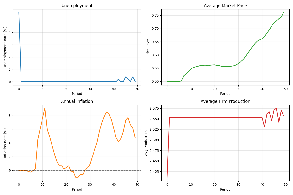
Visualizing Results

Plot key economic indicators over time.

import matplotlib.pyplot as plt

fig, axes = plt.subplots(2, 2, figsize=(12, 8))

# Unemployment rate
ax1 = axes[0, 0]
if len(unemployment) > 0:
    ax1.plot(unemployment * 100, linewidth=2, color="tab:blue")
    ax1.set_ylabel("Unemployment Rate (%)")
    ax1.set_title("Unemployment")
    ax1.grid(True, alpha=0.3)

# Average price
ax2 = axes[0, 1]
if len(avg_price) > 0:
    ax2.plot(avg_price, linewidth=2, color="tab:green")
    ax2.set_ylabel("Price Level")
    ax2.set_title("Average Market Price")
    ax2.grid(True, alpha=0.3)

# Inflation
ax3 = axes[1, 0]
if len(inflation) > 0:
    ax3.plot(inflation * 100, linewidth=2, color="tab:orange")
    ax3.set_ylabel("Inflation Rate (%)")
    ax3.set_title("Annual Inflation")
    ax3.axhline(y=0, color="black", linestyle="--", alpha=0.5)
    ax3.grid(True, alpha=0.3)

# Production - compute mean across firms since data is 2D
ax4 = axes[1, 1]
production_data = results["Producer.production"]
# Average across firms (axis=1) since data is (periods, firms)
avg_production = np.mean(production_data, axis=1)
ax4.plot(avg_production, linewidth=2, color="tab:red")
ax4.set_ylabel("Avg Production")
ax4.set_title("Average Firm Production")
ax4.grid(True, alpha=0.3)

for ax in axes.flat:
    ax.set_xlabel("Period")

plt.tight_layout()
plt.show()

Custom Data Collection

Use a dictionary to specify exactly what data to collect. Keys are role names (or “Economy”), values are True for all variables or a list of specific variable names.

# Collect only specific roles (economy metrics are always included automatically)
custom_results = bam.Simulation.init(n_firms=100, n_households=500, seed=42).run(
    n_periods=30,
    collect={
        "Producer": True,  # All Producer variables
        "Worker": True,  # All Worker variables
        "aggregate": "mean",  # Average across agents
    },
)

print("Custom collection:")
print(f"  Roles collected: {list(custom_results.role_data.keys())}")

Custom collection:
  Roles collected: ['Producer', 'Worker']

Full Agent-Level Data

Dict-form collect returns full per-agent data by default (larger arrays).

# Warning: This collects full arrays - can be memory intensive!
full_results = bam.Simulation.init(n_firms=50, n_households=250, seed=42).run(
    n_periods=20,
    collect={
        "Producer": ["price", "production"],  # Specific variables only
    },
)

prices_full = full_results["Producer.price"]
print(f"Full price data shape: {prices_full.shape}")
print(f"  (periods x firms): ({prices_full.shape[0]} x {prices_full.shape[1]})")

# Access individual firm's price history
firm_0_prices = prices_full[:, 0]
print(f"Firm 0 price history: {firm_0_prices[:5].round(3)}...")

Full price data shape: (20, 50)
  (periods x firms): (20 x 50)
Firm 0 price history: [0.5 0.5 0.5 0.5 0.5]...

Export to pandas DataFrame

Convert results to pandas DataFrames for further analysis. Note: pandas is an optional dependency.

try:
    import pandas

    # Run a new simulation for DataFrame export
    df_results = bam.Simulation.init(n_firms=100, n_households=500, seed=42).run(
        n_periods=50,
        collect=True,
    )

    # Get all data as a single DataFrame (aggregated)
    df = df_results.to_dataframe(aggregate="mean")
    print("Full DataFrame:")
    print(f"  Shape: {df.shape}")
    print(f"  Columns: {list(df.columns)[:5]}...")

    # Get economy metrics only
    df_economy = df_results.economy_metrics
    print("\nEconomy metrics DataFrame:")
    print(df_economy.head())

    # Get specific role data
    df_producer = df_results.get_role_data("Producer", aggregate="mean")
    print(f"\nProducer DataFrame columns: {list(df_producer.columns)}")

except ImportError:
    print("pandas not installed. Install with: pip install pandas")

Full DataFrame:
  Shape: (50, 50)
  Columns: ['Producer.production.mean', 'Producer.production_prev.mean', 'Producer.inventory.mean', 'Producer.expected_demand.mean', 'Producer.desired_production.mean']...

Economy metrics DataFrame:
        avg_price  inflation  n_firm_bankruptcies  n_bank_bankruptcies
period
0          0.5000        0.0                    3                    0
1          0.5000        0.0                    3                    0
2          0.5000        0.0                    3                    0
3          0.5000        0.0                    3                    0
4          0.4993        0.0                    3                    0

Producer DataFrame columns: ['Producer.production.mean', 'Producer.production_prev.mean', 'Producer.inventory.mean', 'Producer.expected_demand.mean', 'Producer.desired_production.mean', 'Producer.labor_productivity.mean', 'Producer.breakeven_price.mean', 'Producer.price.mean', 'Producer.prod_shock.mean', 'Producer.prod_mask_up.mean', 'Producer.prod_mask_dn.mean', 'Producer.price_shock.mean']

Summary Statistics

Get descriptive statistics for all collected metrics.

try:
    import pandas  # noqa: F401 - check if pandas is installed

    summary_results = bam.Simulation.init(n_firms=100, n_households=500, seed=42).run(
        n_periods=100,
        collect=True,
    )

    # Get summary statistics
    summary = summary_results.summary
    print("Summary Statistics:")
    print(summary[["mean", "std", "min", "max"]].round(4))

except ImportError:
    print("pandas not installed for summary statistics")

Summary Statistics:
                                       mean      std       min       max
Producer.production.mean             2.4760   0.1204    2.2038    2.6269
Producer.production_prev.mean        2.4760   0.1204    2.2038    2.6269
Producer.inventory.mean              0.4588   0.2348    0.0000    0.8617
Producer.expected_demand.mean        2.4208   0.1341    2.1307    2.6259
Producer.desired_production.mean     2.4208   0.1341    2.1307    2.6259
Producer.labor_productivity.mean     0.5000   0.0000    0.5000    0.5000
Producer.breakeven_price.mean        0.4973   0.0943    0.0000    0.6197
Producer.price.mean                  0.7392   0.1604    0.5010    0.9675
Producer.prod_shock.mean             0.0500   0.0026    0.0437    0.0585
Producer.prod_mask_up.mean           0.3261   0.2360    0.0100    1.0000
Producer.prod_mask_dn.mean           0.2293   0.1083    0.0000    0.4200
Producer.price_shock.mean            0.0496   0.0027    0.0441    0.0593
Worker.employer.mean                42.2989  13.5160    1.6520   50.4040
Worker.employer_prev.mean           43.9607  12.4924   -1.0000   48.9120
Worker.wage.mean                     0.2339   0.0829    0.0107    0.3503
Worker.periods_left.mean             3.5029   1.9318    0.0600    6.5900
Worker.contract_expired.mean         0.1139   0.2641    0.0000    0.9400
Worker.fired.mean                    0.0022   0.0063    0.0000    0.0360
Worker.job_apps_head.mean           -1.0000   0.0000   -1.0000   -1.0000
Employer.desired_labor.mean          5.1209   0.3911    4.3600    5.9700
Employer.current_labor.mean          4.2857   1.3260    0.3000    5.0000
Employer.wage_offer.mean             0.2646   0.0407    0.1682    0.3259
Employer.wage_bill.mean              1.3187   0.2453    0.8054    1.7740
Employer.n_vacancies.mean            0.2661   0.2427    0.0000    1.1200
Employer.total_funds.mean           12.2919   1.9966    7.7255   15.8609
Employer.wage_shock.mean             0.0110   0.0064    0.0022    0.0267
Borrower.net_worth.mean             12.2919   1.9966    7.7255   15.8609
Borrower.total_funds.mean           12.2919   1.9966    7.7255   15.8609
Borrower.wage_bill.mean              1.3187   0.2453    0.8054    1.7740
Borrower.credit_demand.mean          0.0025   0.0129    0.0000    0.1020
Borrower.projected_fragility.mean    0.0179   0.0581    0.0000    0.4504
Borrower.gross_profit.mean           0.0762   0.1082   -0.0929    0.3913
Borrower.net_profit.mean             0.0760   0.1081   -0.0932    0.3913
Borrower.retained_profit.mean        0.0510   0.1027   -0.1144    0.3521
Borrower.loan_apps_head.mean        -0.1178   1.4605   -1.0000    5.9200
Lender.equity_base.mean              3.9662   1.1033    2.0669    5.0012
Lender.credit_supply.mean           39.6654  11.1486   20.4475   50.0000
Lender.interest_rate.mean            0.0208   0.0006    0.0187    0.0216
Lender.opex_shock.mean               0.0495   0.0092    0.0307    0.0818
Consumer.income.mean                 0.0000   0.0000    0.0000    0.0000
Consumer.savings.mean                0.2682   0.1526    0.1158    0.9335
Consumer.income_to_spend.mean        0.0000   0.0000    0.0000    0.0000
Consumer.propensity.mean             0.7723   0.0247    0.6639    0.8162
Consumer.largest_prod_prev.mean     45.4211   6.8881   33.3360   60.1140
Consumer.shop_visits_head.mean     499.0000   0.0000  499.0000  499.0000
Shareholder.dividends.mean           0.0050   0.0018    0.0018    0.0086
avg_price                            0.7325   0.1577    0.4970    0.9519
inflation                            0.0198   0.0333   -0.0424    0.0771
n_firm_bankruptcies                  3.9200   2.7217    0.0000   11.0000
n_bank_bankruptcies                  0.0700   0.2564    0.0000    1.0000

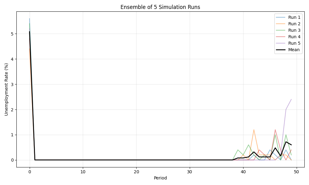
Comparing Multiple Simulation Runs

Run multiple simulations and compare their results.

# Run with different random seeds
n_runs = 5
all_unemployment = []

print("Running ensemble of simulations...")
for i in range(n_runs):
    run_results = bam.Simulation.init(n_firms=100, n_households=500, seed=42 + i).run(
        n_periods=50,
        collect={
            "Worker": ["employed"],
            "capture_timing": {"Worker.employed": "firms_run_production"},
        },
    )
    # Calculate unemployment from Worker employed data
    unemp_rate = calc_unemployment_rate(run_results["Worker.employed"])
    all_unemployment.append(unemp_rate)

# Plot ensemble results
if all_unemployment:
    fig, ax = plt.subplots(figsize=(10, 6))

    for i, unemp in enumerate(all_unemployment):
        ax.plot(bam.ops.multiply(unemp, 100), alpha=0.5, label=f"Run {i + 1}")

    # Calculate and plot mean unemployment across runs
    # Stack arrays and compute mean along axis 0
    stacked = bam.ops.asarray([list(u) for u in all_unemployment])
    mean_unemployment = bam.ops.multiply(bam.ops.mean(stacked, axis=0), 100)
    ax.plot(mean_unemployment, "k-", linewidth=2, label="Mean")

    ax.set_xlabel("Period")
    ax.set_ylabel("Unemployment Rate (%)")
    ax.set_title(f"Ensemble of {n_runs} Simulation Runs")
    ax.legend(loc="upper right")
    ax.grid(True, alpha=0.3)
    plt.tight_layout()
    plt.show()

    # Summary across runs
    final_rates = bam.ops.asarray([unemp[-1] * 100 for unemp in all_unemployment])
    print("\nFinal unemployment rates:")
    print(f"  Mean: {bam.ops.mean(final_rates):.2f}%")
    print(f"  Std:  {bam.ops.std(final_rates):.2f}%")
    print(f"  Range: {bam.ops.min(final_rates):.2f}% - {bam.ops.max(final_rates):.2f}%")

Running ensemble of simulations...

Final unemployment rates:
  Mean: 0.36%
  Std:  0.37%
  Range: 0.00% - 1.00%

Collecting Relationship Data

Relationships (like LoanBook) can be collected alongside role data. Unlike roles, relationships are opt-in only and NOT included with collect=True.

# Manually add some loans to demonstrate relationship data collection
rel_sim = bam.Simulation.init(n_firms=50, n_households=250, seed=42)
loans = rel_sim.get_relationship("LoanBook")
loans.append_loans_for_lender(
    lender_idx=np.intp(0),
    borrower_indices=np.array([0, 1, 2, 3, 4], dtype=np.int64),
    amount=np.array([1000.0, 1500.0, 2000.0, 500.0, 750.0]),
    rate=np.array([0.02, 0.03, 0.025, 0.018, 0.022]),
)

rel_results = rel_sim.run(
    n_periods=20,
    collect={
        "Producer": ["price"],  # Role data
        "LoanBook": ["principal", "rate", "debt"],  # Relationship data
        "aggregate": "sum",  # Sum across all active loans
    },
)

print("Relationship data collection:")
print(f"  Available: {rel_results.available()}")

# Access via bracket notation
total_principal = rel_results["LoanBook.principal"]
print(f"  Total principal over time shape: {total_principal.shape}")
print(f"  Initial total principal: {total_principal[0]:.2f}")

# Access via get()
total_debt = rel_results.get("LoanBook", "debt")
print(f"  Total debt (last period): {total_debt[-1]:.2f}")

Relationship data collection:
  Available: ['Economy.avg_price', 'Economy.inflation', 'Economy.n_bank_bankruptcies', 'Economy.n_firm_bankruptcies', 'LoanBook.debt', 'LoanBook.principal', 'LoanBook.rate', 'Producer.price']
  Total principal over time shape: (20,)
  Initial total principal: 0.00
  Total debt (last period): 0.00

Analyzing Loan Distribution

Without aggregation (the default for dict-form collect), you get full edge data per period as variable-length arrays. Useful for analyzing distributions but cannot be exported to DataFrame.

loan_dist_sim = bam.Simulation.init(n_firms=50, n_households=250, seed=42)
loans = loan_dist_sim.get_relationship("LoanBook")
# Add loans with varying amounts
loans.append_loans_for_lender(
    lender_idx=np.intp(0),
    borrower_indices=np.array([0, 1, 2], dtype=np.int64),
    amount=np.array([100.0, 200.0, 300.0]),
    rate=np.array([0.02, 0.03, 0.025]),
)

dist_results = loan_dist_sim.run(
    n_periods=5,
    collect={
        "LoanBook": ["principal"],  # Full edge data (variable-length per period)
    },
)

principal_per_period = dist_results["LoanBook.principal"]
print("\nLoan distribution (full per-edge data):")
print(f"  Type: {type(principal_per_period).__name__}")
print(f"  Number of periods: {len(principal_per_period)}")
if principal_per_period:
    print(f"  Period 0 loans: {len(principal_per_period[0])} active")
    print(f"  Period 0 principals: {principal_per_period[0]}")

Loan distribution (full per-edge data):
  Type: list
  Number of periods: 5
  Period 0 loans: 0 active
  Period 0 principals: []

Key Takeaways

Basic collection:

• Use collect=True (the default) for full per-agent data collection

• Economy metrics are always collected automatically

• Use collect={"Producer": ["price"]} for specific variables

• Use True for all variables: {"Worker": True}

Data access (primary API):

• results["Producer.price"] – bracket notation (recommended)

• results.Producer.price – attribute access (interactive use)

• results.get("Producer", "price") – programmatic access

• results.get("Producer", "price", aggregate="mean") – with aggregation

• results.available() – discover all collected variables

Per-agent data and capture timing:

• Dict-form collect returns full per-agent data by default (shape: periods x agents)

• Use capture_timing to control when variables are captured during each period

• Example: "capture_timing": {"Worker.employed": "firms_run_production"}

Computing derived metrics:

• Unemployment rate can be computed from Worker.employed: 1.0 - np.mean(employed.astype(float), axis=1)

• When computing from per-agent data, aggregate across agents with axis=1

Relationship data:

• Relationships (like LoanBook) are opt-in: use "LoanBook": ["principal"]

• NOT included with collect=True (must specify explicitly)

• Aggregations: sum (total), mean (average), std (variation)

• Without aggregation (default): list of variable-length arrays (can’t export to DataFrame)

• Access via results["LoanBook.principal"] or results.get("LoanBook", "principal")

Legacy access (still works):

• results.economy_data, results.role_data, results.relationship_data

• results.data for unified dict access (includes “Economy” key and relationships)

• Export to pandas with to_dataframe() for further analysis

• Get quick statistics with results.summary