Growth+ Model Extension

This example implements the Growth+ extension from chapter 3.8 of Macroeconomics from the Bottom-up, demonstrating endogenous productivity growth based on R&D investment.

Key Equations

Productivity Evolution (Equation 3.15):

\[\alpha_{t+1} = \alpha_t + z_t\]

Where \(z_t \sim \text{Exponential}(\mu)\) represents the productivity increment drawn from an exponential distribution with scale parameter \(\mu\).

R&D Intensity (expected productivity gain):

\[\mu = \sigma \cdot \frac{\pi}{p \cdot Y}\]

This example demonstrates:

• Defining custom roles with the @role decorator

• Creating custom events with the @event decorator

• Using pipeline hooks via @event(after=...) for declarative event positioning

• Attaching custom roles to simulations via sim.use_role()

For detailed validation with bounds and statistical annotations, run:

python -m validation.scenarios.growth_plus

Import Dependencies

We import BAM Engine and the decorators needed to define custom components.

import bamengine as bam
from bamengine import Float, event, ops, role

Define Custom Role: RnD

The RnD role tracks R&D-related state for each firm.

@role
class RnD:
    """R&D state for Growth+ extension."""

    sigma: Float  # R&D share of profits
    rnd_intensity: Float  # Expected productivity gain (mu)
    productivity_increment: Float  # Actual productivity increment (z)
    fragility: Float  # Financial fragility (wage_bill / net_worth)

Define Custom Events

Three events implement the Growth+ mechanism.

@event(name="firms_compute_rnd_intensity", after="firms_validate_debt_commitments")
class FirmsComputeRnDIntensity:
    """Compute R&D share and intensity for firms."""

    def execute(self, sim: bam.Simulation) -> None:
        bor = sim.get_role("Borrower")
        prod = sim.get_role("Producer")
        emp = sim.get_role("Employer")
        rnd = sim.get_role("RnD")

        sigma_min, sigma_max, sigma_decay = (
            sim.sigma_min,
            sim.sigma_max,
            sim.sigma_decay,
        )

        eps = 1e-10
        safe_net_worth = ops.where(ops.greater(bor.net_worth, eps), bor.net_worth, eps)
        fragility = ops.divide(emp.wage_bill, safe_net_worth)
        ops.assign(rnd.fragility, fragility)

        decay_factor = ops.exp(ops.multiply(sigma_decay, fragility))
        sigma = ops.add(sigma_min, ops.multiply(sigma_max - sigma_min, decay_factor))
        sigma = ops.where(ops.greater(bor.net_profit, 0.0), sigma, 0.0)
        ops.assign(rnd.sigma, sigma)

        revenue = ops.multiply(prod.price, prod.production)
        safe_revenue = ops.where(ops.greater(revenue, eps), revenue, eps)
        mu = ops.divide(ops.multiply(sigma, bor.net_profit), safe_revenue)
        mu = ops.where(ops.greater(mu, 0.0), mu, 0.0)
        ops.assign(rnd.rnd_intensity, mu)


@event(after="firms_compute_rnd_intensity")
class FirmsApplyProductivityGrowth:
    """Apply productivity growth based on R&D."""

    def execute(self, sim: bam.Simulation) -> None:
        prod = sim.get_role("Producer")
        rnd = sim.get_role("RnD")

        z = ops.zeros(sim.n_firms)
        active = ops.greater(rnd.rnd_intensity, 0.0)
        if ops.any(active):
            z[active] = sim.rng.exponential(scale=rnd.rnd_intensity[active])

        ops.assign(rnd.productivity_increment, z)
        ops.assign(prod.labor_productivity, ops.add(prod.labor_productivity, z))


@event(after="firms_apply_productivity_growth")
class FirmsDeductRnDExpenditure:
    """Adjust net profit for R&D expenditure."""

    def execute(self, sim: bam.Simulation) -> None:
        bor = sim.get_role("Borrower")
        rnd = sim.get_role("RnD")
        new_net_profit = ops.multiply(bor.net_profit, ops.subtract(1.0, rnd.sigma))
        ops.assign(bor.net_profit, new_net_profit)

Initialize Simulation

Create a simulation using extra parameters for the Growth+ extension and attach the RnD role and events.

sim = bam.Simulation.init(
    # Growth+ parameters
    sigma_min=0.0,
    sigma_max=0.1,
    sigma_decay=-1.0,
    # Seed
    seed=0,
)

sim.use_role(RnD)
sim.use_events(
    FirmsComputeRnDIntensity, FirmsApplyProductivityGrowth, FirmsDeductRnDExpenditure
)
print(f"Growth+ simulation: {sim.n_firms} firms, {sim.n_households} households")

Growth+ simulation: 100 firms, 500 households

Run Simulation

Collect per-agent data with capture timing matching the validation scenario.

COLLECT_CONFIG = {
    "Producer": ["production", "labor_productivity", "price", "inventory"],
    "Worker": ["wage", "employed"],
    "Employer": ["n_vacancies"],
    "Borrower": ["net_worth"],
    "Consumer": ["income_to_spend"],
    "LoanBook": ["principal", "rate", "source_ids"],
    "capture_timing": {
        # Capture wages after workers receive them
        "Worker.wage": "firms_run_production",
        # Employment status after production completes
        "Worker.employed": "firms_run_production",
        # Production output after firms run production
        "Producer.production": "firms_run_production",
        # Productivity after R&D growth is applied (captures the increment)
        "Producer.labor_productivity": "firms_apply_productivity_growth",
        # Price after planning phase sets it
        "Producer.price": "firms_plan_price",
        # Inventory after consumers finish purchasing
        "Producer.inventory": "consumers_finalize_purchases",
        # Vacancies right after firms decide them
        "Employer.n_vacancies": "firms_decide_vacancies",
        # Net worth after production (before bankruptcy may reset it)
        "Borrower.net_worth": "firms_run_production",
        # Consumer budget after it's decided
        "Consumer.income_to_spend": "consumers_decide_income_to_spend",
        # Loan data after credit market matching
        "LoanBook.principal": "credit_market_round",
        "LoanBook.rate": "credit_market_round",
        "LoanBook.source_ids": "credit_market_round",
    },
}
results = sim.run(collect=COLLECT_CONFIG)
print(f"Completed: {results.metadata['runtime_seconds']:.2f}s")

Completed: 5.72s

Compute Metrics

Compute macro indicators and financial dynamics from the simulation results.

import numpy as np

burn_in = 500
n_periods = sim.n_periods
EPS = 1e-9

# Extract raw data from results
avg_price = results["Economy.avg_price"]
production = results.get("Producer", "production")
productivity = results.get("Producer", "labor_productivity")
prices = results.get("Producer", "price")
inventory = results.get("Producer", "inventory")
wages = results.get("Worker", "wage")
employed_arr = results.get("Worker", "employed")
n_vacancies = results.get("Employer", "n_vacancies")
net_worth = results.get("Borrower", "net_worth")
consumer_budget = results.get("Consumer", "income_to_spend")
loan_principals = results["LoanBook.principal"]
loan_rates = results["LoanBook.rate"]
bankruptcies = np.array(results["Economy.n_firm_bankruptcies"])

# Compute total production (GDP)
gdp = ops.sum(production, axis=1)

# Unemployment rate
unemployment = 1 - ops.mean(employed_arr.astype(float), axis=1)

# Log GDP
log_gdp = ops.log(gdp + 1e-10)

# Inflation
inflation = results["Economy.inflation"]

# Average wage for employed workers
employed_wages_sum = ops.sum(ops.where(employed_arr, wages, 0.0), axis=1)
employed_count = ops.sum(employed_arr, axis=1)
avg_wage = ops.where(
    ops.greater(employed_count, 0),
    ops.divide(employed_wages_sum, employed_count),
    0.0,
)

# Real wage
real_wage = ops.divide(avg_wage, avg_price)

# Production-weighted average productivity
weighted_prod = ops.sum(ops.multiply(productivity, production), axis=1)
avg_productivity = ops.divide(weighted_prod, gdp)

# Wage inflation for Phillips curve
wage_inflation = ops.divide(
    avg_wage[1:] - avg_wage[:-1],
    ops.where(ops.greater(avg_wage[:-1], 0), avg_wage[:-1], 1.0),
)

# GDP growth for Okun curve
gdp_growth = ops.divide(gdp[1:] - gdp[:-1], gdp[:-1])

# Unemployment growth for Okun curve
unemployment_growth = ops.divide(
    unemployment[1:] - unemployment[:-1],
    ops.where(ops.greater(unemployment[:-1], 0), unemployment[:-1], 1.0),
)

# Vacancy rate
total_vacancies = ops.sum(n_vacancies, axis=1)
vacancy_rate = ops.divide(total_vacancies, sim.n_households)

# Final period firm production
prod = sim.get_role("Producer")
final_production = prod.production.copy()

# Correlations
phillips_corr = np.corrcoef(unemployment[burn_in:], wage_inflation[burn_in - 1 :])[0, 1]
okun_corr = np.corrcoef(unemployment_growth[burn_in - 1 :], gdp_growth[burn_in - 1 :])[
    0, 1
]
beveridge_corr = np.corrcoef(unemployment[burn_in:], vacancy_rate[burn_in:])[0, 1]

prod_growth = (avg_productivity[-1] - avg_productivity[burn_in]) / avg_productivity[
    burn_in
]


# Recession detection
def detect_recessions(
    log_gdp_series, window=5, threshold=0.02, min_gap=10, min_duration=15
):
    """Detect recessions as sustained drawdowns from smoothed GDP peaks."""
    kernel = np.ones(window) / window
    smoothed = np.convolve(log_gdp_series, kernel, mode="same")
    running_max = np.maximum.accumulate(smoothed)
    drawdown = running_max - smoothed
    mask = drawdown > threshold
    if np.any(mask):
        # Bridge short gaps between nearby recessions
        padded = np.concatenate([[False], mask, [False]])
        starts = np.where(padded[1:] & ~padded[:-1])[0]
        ends = np.where(~padded[1:] & padded[:-1])[0]
        for i in range(len(ends) - 1):
            if starts[i + 1] - ends[i] < min_gap:
                mask[ends[i] : starts[i + 1]] = True
        # Remove recessions shorter than min_duration
        padded = np.concatenate([[False], mask, [False]])
        starts = np.where(padded[1:] & ~padded[:-1])[0]
        ends = np.where(~padded[1:] & padded[:-1])[0]
        for s, e in zip(starts, ends, strict=True):
            if e - s < min_duration:
                mask[s:e] = False
    return mask


recession_mask = detect_recessions(log_gdp)

# Financial dynamics
real_interest_rate = np.zeros(n_periods)
for t in range(n_periods):
    principals_t = loan_principals[t]
    rates_t = loan_rates[t]
    if len(principals_t) > 0 and np.sum(principals_t) > 0:
        weighted_nominal = float(np.sum(rates_t * principals_t) / np.sum(principals_t))
    else:
        weighted_nominal = sim.r_bar
    real_interest_rate[t] = weighted_nominal - inflation[t]

total_wage_bill = ops.sum(wages * employed_arr.astype(float), axis=1)
total_net_worth = ops.sum(net_worth, axis=1)
safe_total_nw = ops.where(ops.greater(total_net_worth, EPS), total_net_worth, EPS)
financial_fragility = ops.divide(total_wage_bill, safe_total_nw)

safe_gdp = ops.where(ops.greater(gdp, EPS), gdp, EPS)
total_demand = ops.sum(consumer_budget, axis=1)
market_clearing_price = ops.divide(total_demand, safe_gdp)
price_ratio = ops.divide(avg_price, market_clearing_price)

# Price dispersion: production-weighted CV
safe_prod = np.where(production > 0, production, 0.0)
prod_sum = np.sum(safe_prod, axis=1, keepdims=True)
prod_weights = safe_prod / np.where(prod_sum > EPS, prod_sum, EPS)
weighted_price_mean = np.sum(prod_weights * prices, axis=1, keepdims=True)
weighted_price_var = np.sum(prod_weights * (prices - weighted_price_mean) ** 2, axis=1)
weighted_price_std = np.sqrt(np.maximum(weighted_price_var, 0.0))
w_mean_flat = weighted_price_mean.squeeze()
safe_w_mean = np.where(w_mean_flat > EPS, w_mean_flat, EPS)
price_dispersion = weighted_price_std / safe_w_mean

# Equity dispersion: std / abs(mean) with EPS
nw_mean = ops.mean(net_worth, axis=1)
equity_dispersion = ops.divide(
    ops.std(net_worth, axis=1),
    ops.where(ops.greater(np.abs(nw_mean), EPS), np.abs(nw_mean), EPS),
)

# Sales dispersion: price * (production - inventory)
qty_sold = np.subtract(production, inventory)
sales = ops.multiply(prices, qty_sold)
sales_mean = ops.mean(sales, axis=1)
sales_dispersion = ops.divide(
    ops.std(sales, axis=1),
    ops.where(ops.greater(np.abs(sales_mean), EPS), np.abs(sales_mean), EPS),
)

# Output growth rates (aggregate GDP, post-burn-in)
gdp_after_burnin = gdp[burn_in:]
output_growth_rates = np.diff(gdp_after_burnin) / gdp_after_burnin[:-1]

# Net worth growth rates (final two periods, valid firms)
nw_prev = net_worth[-2]
nw_final = net_worth[-1]
valid_firms = (nw_prev > 0) & (nw_final > 0)
nw_prev_valid = nw_prev[valid_firms]
nw_final_valid = nw_final[valid_firms]
networth_growth_rates = (nw_final_valid - nw_prev_valid) / nw_prev_valid

# Exclude re-entries (bankruptcy respawns cause |growth| >> 100%)
reentry_mask = np.abs(networth_growth_rates) <= 1.0
networth_growth_rates = networth_growth_rates[reentry_mask]

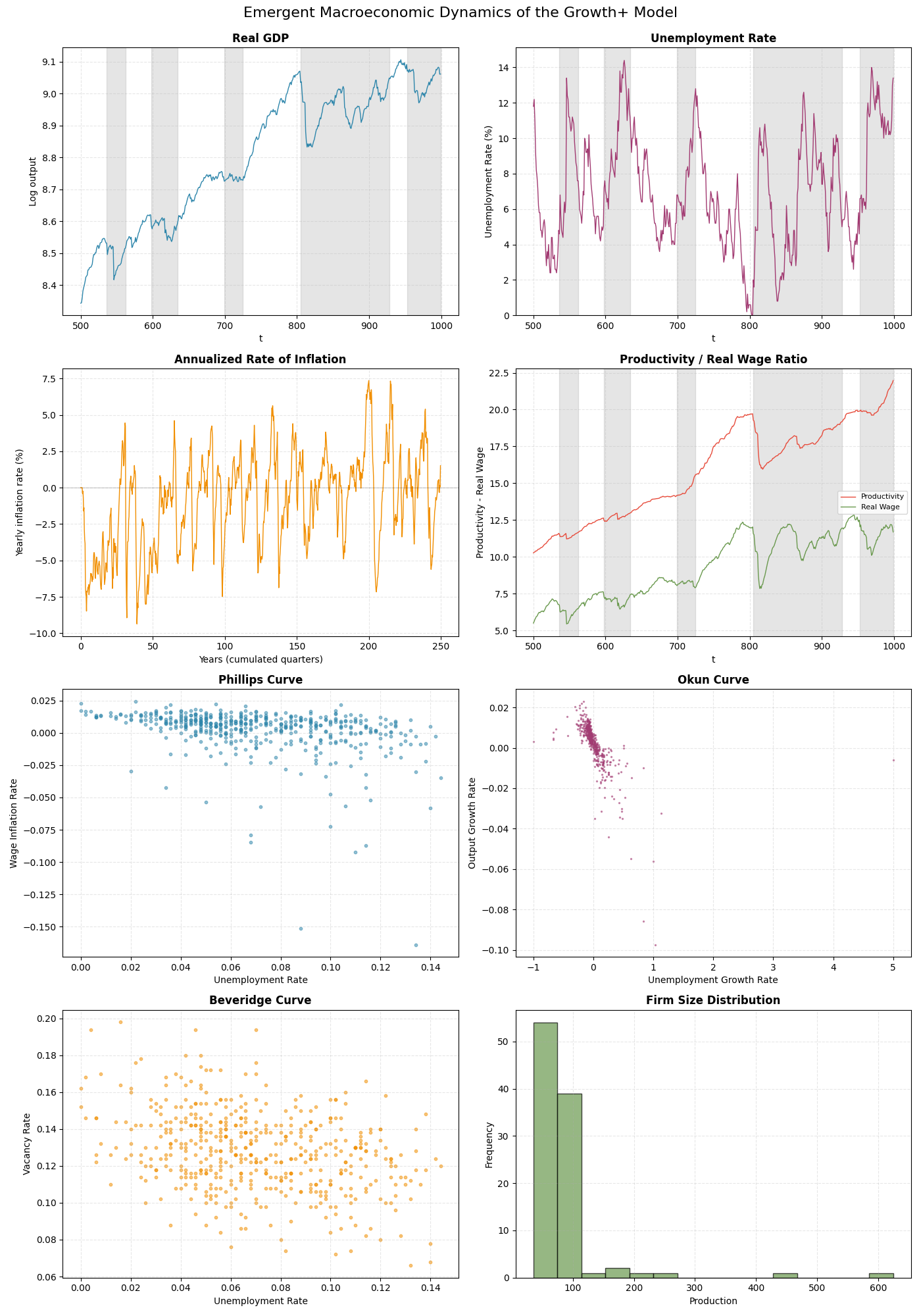
print(f"\nKey metrics (after {burn_in}-period burn-in):")
print(f"  Unemployment: {np.mean(unemployment[burn_in:]) * 100:.1f}%")
print(f"  Inflation: {np.mean(inflation[burn_in:]) * 100:.1f}%")
print(f"  Productivity growth: {prod_growth * 100:.0f}%")
print(f"  Phillips correlation: {phillips_corr:.2f}")
print(f"  Okun correlation: {okun_corr:.2f}")
print(f"  Beveridge correlation: {beveridge_corr:.2f}")

Key metrics (after 500-period burn-in):
  Unemployment: 7.0%
  Inflation: 0.2%
  Productivity growth: 114%
  Phillips correlation: -0.33
  Okun correlation: -0.53
  Beveridge correlation: -0.33

Visualize Results (Macro Dynamics)

4x2 figure showing time series with recession bands and macroeconomic curves.

import matplotlib.pyplot as plt


def add_recession_bands(ax, periods, mask):
    """Shade recession episodes on a time-series axis."""
    if not np.any(mask):
        return
    in_rec = False
    start_idx = 0
    for i, is_rec in enumerate(mask):
        if is_rec and not in_rec:
            start_idx = i
            in_rec = True
        elif not is_rec and in_rec:
            ax.axvspan(periods[start_idx], periods[i - 1], alpha=0.2, color="gray")
            in_rec = False
    if in_rec:
        ax.axvspan(periods[start_idx], periods[-1], alpha=0.2, color="gray")


periods = ops.arange(burn_in, n_periods)
fig, axes = plt.subplots(4, 2, figsize=(14, 20))
fig.suptitle(
    "Emergent Macroeconomic Dynamics of the Growth+ Model", fontsize=16, y=0.995
)

# Panel (0,0): Log Real GDP
ax = axes[0, 0]
add_recession_bands(ax, periods, recession_mask[burn_in:])
ax.plot(periods, log_gdp[burn_in:], linewidth=1, color="#2E86AB")
ax.set_title("Real GDP", fontsize=12, fontweight="bold")
ax.set_ylabel("Log output")
ax.set_xlabel("t")
ax.grid(True, linestyle="--", alpha=0.3)

# Panel (0,1): Unemployment Rate
ax = axes[0, 1]
add_recession_bands(ax, periods, recession_mask[burn_in:])
ax.plot(periods, unemployment[burn_in:] * 100, linewidth=1, color="#A23B72")
ax.set_title("Unemployment Rate", fontsize=12, fontweight="bold")
ax.set_ylabel("Unemployment Rate (%)")
ax.set_xlabel("t")
ax.set_ylim(bottom=0)
ax.grid(True, linestyle="--", alpha=0.3)

# Panel (1,0): Inflation Rate (all periods, cumulated years)
ax = axes[1, 0]
years = ops.arange(0, n_periods) / 4
ax.plot(years, inflation * 100, linewidth=1, color="#F18F01")
ax.axhline(0, color="black", linestyle="-", alpha=0.3, linewidth=0.5)
ax.set_title("Annualized Rate of Inflation", fontsize=12, fontweight="bold")
ax.set_ylabel("Yearly inflation rate (%)")
ax.set_xlabel("Years (cumulated quarters)")
ax.grid(True, linestyle="--", alpha=0.3)

# Panel (1,1): Productivity and Real Wage
ax = axes[1, 1]
add_recession_bands(ax, periods, recession_mask[burn_in:])
ax.plot(
    periods,
    avg_productivity[burn_in:],
    linewidth=1,
    color="#E74C3C",
    label="Productivity",
)
ax.plot(periods, real_wage[burn_in:], linewidth=1, color="#6A994E", label="Real Wage")
ax.set_title("Productivity / Real Wage Ratio", fontsize=12, fontweight="bold")
ax.set_ylabel("Productivity - Real Wage")
ax.set_xlabel("t")
ax.legend(loc="center right", fontsize=8)
ax.grid(True, linestyle="--", alpha=0.3)

# Panel (2,0): Phillips Curve
ax = axes[2, 0]
ax.scatter(
    unemployment[burn_in:],
    wage_inflation[burn_in - 1 :],
    s=10,
    alpha=0.5,
    color="#2E86AB",
)
ax.set_title("Phillips Curve", fontsize=12, fontweight="bold")
ax.set_xlabel("Unemployment Rate")
ax.set_ylabel("Wage Inflation Rate")
ax.grid(True, linestyle="--", alpha=0.3)

# Panel (2,1): Okun Curve
ax = axes[2, 1]
ax.scatter(
    unemployment_growth[burn_in - 1 :],
    gdp_growth[burn_in - 1 :],
    s=2,
    alpha=0.5,
    color="#A23B72",
)
ax.set_title("Okun Curve", fontsize=12, fontweight="bold")
ax.set_xlabel("Unemployment Growth Rate")
ax.set_ylabel("Output Growth Rate")
ax.grid(True, linestyle="--", alpha=0.3)

# Panel (3,0): Beveridge Curve
ax = axes[3, 0]
ax.scatter(
    unemployment[burn_in:], vacancy_rate[burn_in:], s=10, alpha=0.5, color="#F18F01"
)
ax.set_title("Beveridge Curve", fontsize=12, fontweight="bold")
ax.set_xlabel("Unemployment Rate")
ax.set_ylabel("Vacancy Rate")
ax.grid(True, linestyle="--", alpha=0.3)

# Panel (3,1): Firm Size Distribution
ax = axes[3, 1]
ax.hist(final_production, bins=15, edgecolor="black", alpha=0.7, color="#6A994E")
ax.set_title("Firm Size Distribution", fontsize=12, fontweight="bold")
ax.set_xlabel("Production")
ax.set_ylabel("Frequency")
ax.grid(True, linestyle="--", alpha=0.3)

plt.tight_layout()
plt.show()

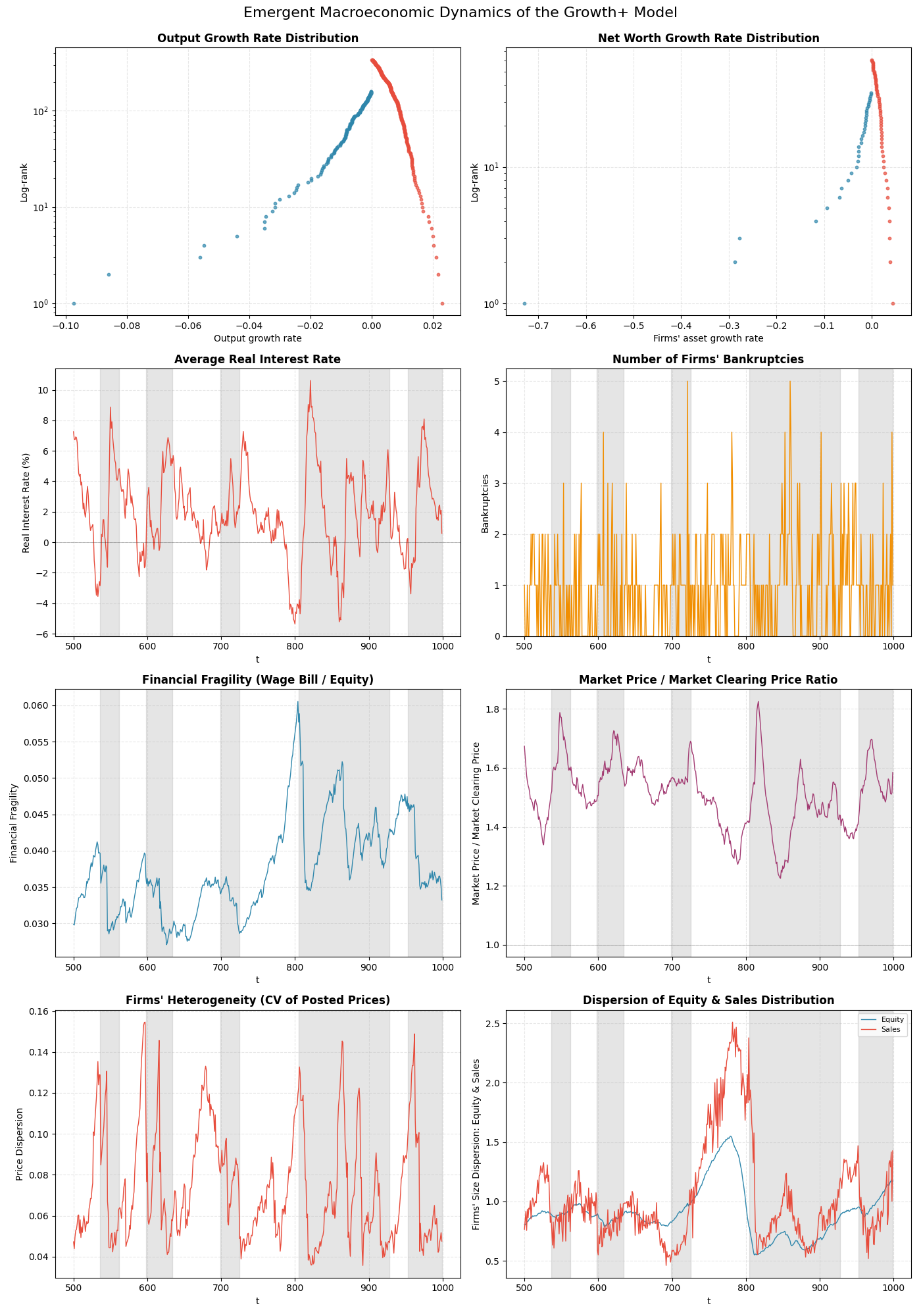
Visualize Financial Dynamics

4x2 figure showing growth distributions, interest rates, and financial indicators.

fig2, axes2 = plt.subplots(4, 2, figsize=(14, 20))
fig2.suptitle(
    "Emergent Macroeconomic Dynamics of the Growth+ Model", fontsize=16, y=0.995
)

# Panel (0,0): Output Growth Rate Distribution (log-rank)
ax = axes2[0, 0]
filtered = output_growth_rates[np.isfinite(output_growth_rates)]
negative = filtered[filtered < 0]
positive = filtered[filtered >= 0]
neg_sorted = np.sort(negative)
neg_ranks = np.arange(1, len(neg_sorted) + 1)
pos_sorted = np.sort(positive)[::-1]
pos_ranks = np.arange(1, len(pos_sorted) + 1)
ax.scatter(neg_sorted, neg_ranks, s=10, alpha=0.7, color="#2E86AB")
ax.scatter(pos_sorted, pos_ranks, s=10, alpha=0.7, color="#E74C3C")
ax.set_yscale("log")
ax.set_title("Output Growth Rate Distribution", fontsize=12, fontweight="bold")
ax.set_xlabel("Output growth rate")
ax.set_ylabel("Log-rank")
ax.grid(True, linestyle="--", alpha=0.3)

# Panel (0,1): Net Worth Growth Rate Distribution (log-rank)
ax = axes2[0, 1]
filtered = networth_growth_rates[np.isfinite(networth_growth_rates)]
negative = filtered[filtered < 0]
positive = filtered[filtered >= 0]
neg_sorted = np.sort(negative)
neg_ranks = np.arange(1, len(neg_sorted) + 1)
pos_sorted = np.sort(positive)[::-1]
pos_ranks = np.arange(1, len(pos_sorted) + 1)
ax.scatter(neg_sorted, neg_ranks, s=10, alpha=0.7, color="#2E86AB")
ax.scatter(pos_sorted, pos_ranks, s=10, alpha=0.7, color="#E74C3C")
ax.set_yscale("log")
ax.set_title("Net Worth Growth Rate Distribution", fontsize=12, fontweight="bold")
ax.set_xlabel("Firms' asset growth rate")
ax.set_ylabel("Log-rank")
ax.grid(True, linestyle="--", alpha=0.3)

# Panel (1,0): Real Interest Rate
ax = axes2[1, 0]
add_recession_bands(ax, periods, recession_mask[burn_in:])
ax.plot(periods, real_interest_rate[burn_in:] * 100, linewidth=1, color="#E74C3C")
ax.axhline(0, color="black", linestyle="-", alpha=0.3, linewidth=0.5)
ax.set_title("Average Real Interest Rate", fontsize=12, fontweight="bold")
ax.set_ylabel("Real Interest Rate (%)")
ax.set_xlabel("t")
ax.grid(True, linestyle="--", alpha=0.3)

# Panel (1,1): Firm Bankruptcies
ax = axes2[1, 1]
add_recession_bands(ax, periods, recession_mask[burn_in:])
ax.plot(periods, bankruptcies[burn_in:], linewidth=1, color="#F18F01")
ax.set_title("Number of Firms' Bankruptcies", fontsize=12, fontweight="bold")
ax.set_ylabel("Bankruptcies")
ax.set_xlabel("t")
ax.set_ylim(bottom=0)
ax.grid(True, linestyle="--", alpha=0.3)

# Panel (2,0): Financial Fragility
ax = axes2[2, 0]
add_recession_bands(ax, periods, recession_mask[burn_in:])
ax.plot(periods, financial_fragility[burn_in:], linewidth=1, color="#2E86AB")
ax.set_title("Financial Fragility (Wage Bill / Equity)", fontsize=12, fontweight="bold")
ax.set_ylabel("Financial Fragility")
ax.set_xlabel("t")
ax.grid(True, linestyle="--", alpha=0.3)

# Panel (2,1): Price Ratio
ax = axes2[2, 1]
add_recession_bands(ax, periods, recession_mask[burn_in:])
ax.plot(periods, price_ratio[burn_in:], linewidth=1, color="#A23B72")
ax.axhline(1, color="black", linestyle="-", alpha=0.3, linewidth=0.5)
ax.set_title(
    "Market Price / Market Clearing Price Ratio", fontsize=12, fontweight="bold"
)
ax.set_ylabel("Market Price / Market Clearing Price")
ax.set_xlabel("t")
ax.grid(True, linestyle="--", alpha=0.3)

# Panel (3,0): Price Dispersion (CV)
ax = axes2[3, 0]
add_recession_bands(ax, periods, recession_mask[burn_in:])
ax.plot(periods, price_dispersion[burn_in:], linewidth=1, color="#E74C3C")
ax.set_title(
    "Firms' Heterogeneity (CV of Posted Prices)", fontsize=12, fontweight="bold"
)
ax.set_ylabel("Price Dispersion")
ax.set_xlabel("t")
ax.grid(True, linestyle="--", alpha=0.3)

# Panel (3,1): Equity & Sales Dispersion
ax = axes2[3, 1]
add_recession_bands(ax, periods, recession_mask[burn_in:])
ax.plot(
    periods,
    equity_dispersion[burn_in:],
    linewidth=1,
    color="#2E86AB",
    label="Equity",
)
ax.plot(
    periods,
    sales_dispersion[burn_in:],
    linewidth=1,
    color="#E74C3C",
    label="Sales",
)
ax.set_title(
    "Dispersion of Equity & Sales Distribution", fontsize=12, fontweight="bold"
)
ax.set_ylabel("Firms' Size Dispersion: Equity & Sales")
ax.set_xlabel("t")
ax.legend(loc="upper right", fontsize=8)
ax.grid(True, linestyle="--", alpha=0.3)

plt.tight_layout()
plt.show()

Alternative: Extension Bundle

The above example defines all R&D components inline for educational purposes. For convenience, the pre-built RND bundle activates everything in one call:

from extensions.rnd import RND, RND_COLLECT

sim = bam.Simulation.init(seed=0)
sim.use(RND)
results = sim.run(collect=RND_COLLECT)